Configuration Walkthrough

Apstra: Configure Apstra Server and Apstra ZTP Server

A configuration wizard launches upon connecting to the Apstra server VM for the first time. At this point, passwords for the Apstra server, Apstra UI, and network configuration can be configured. For more information about installation, refer to the Juniper Apstra User Guide.

Apstra: Onboard the devices into Apstra

There are two methods for adding Juniper devices into Apstra for management: manually or in bulk using ZTP.

To add devices manually (recommended):

• In the Apstra UI navigate to Devices > Agents > Create Offbox Agents.

This requires that the devices are preconfigured with a root password, a management-instance [edit system], management IP, and proper static routing if needed, as well as ssh Netconf, so that they can be accessed and configured by Apstra.

To add devices via ZTP:

• From the Apstra ZTP server, follow the ZTP steps described in the Juniper Apstra User Guide.

For this 5-stage JVD setup, a root password and management IPs were already configured on all switches prior to adding the devices to Apstra. To add switches to Apstra, first log into the Apstra Web UI, choose a method of device addition as per above, and provide the appropriate username and password preconfigured for those devices.

Note:

Apstra imports the configuration from the devices into a baseline configuration called pristine configuration, which is a clean, minimal configuration, and is free of any pre-existing settings that could interfere with the intended network design managed by Apstra.

Apstra ignores the Junos configuration ‘groups’ stanza and does not validate any group configuration listed in the inheritance model, refer to the configuration groups usage guide.

It is best practice to avoid setting loopbacks, interfaces (except management interface), routing-instances (except management-instance) or any other settings as part of this baseline configuration.Apstra sets the protocols LLDP and RSTP when the device is successfully Acknowledged.

To onboard the devices, follow these steps:

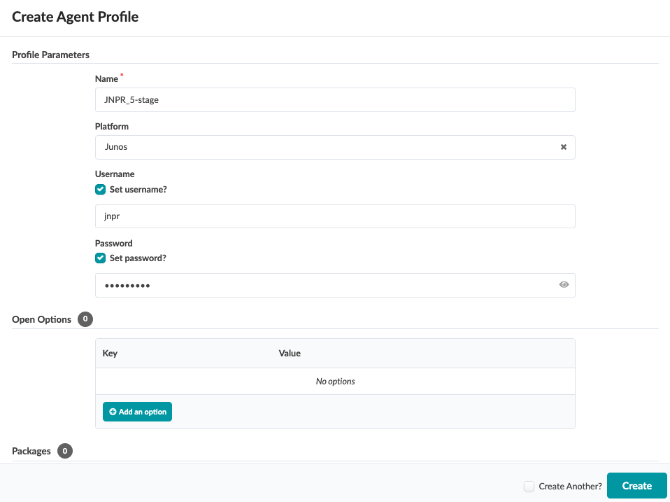
1) Apstra Web UI: Create Agent Profile

For the purposes of this JVD, the same username and password are used across all devices. Thus, only one Apstra Agent Profile is needed to onboard all the devices, making the process more efficient.

To create an Agent Profile, navigate to Devices > Agent Profiles and then click on Create Agent Profile.

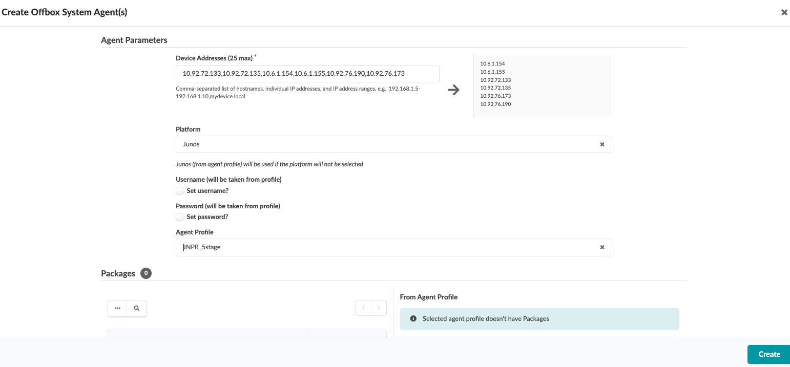
2) Apstra Web UI: Add Range of IP Addresses for Onboarding Devices

An IP address range can be provided to bulk onboard devices in Apstra. The ranges shown in the example below are shown for demonstration purposes only.

To onboard devices, navigate to Devices > Managed Devices and then click on Create Offbox Agents (for Junos OS devices only)

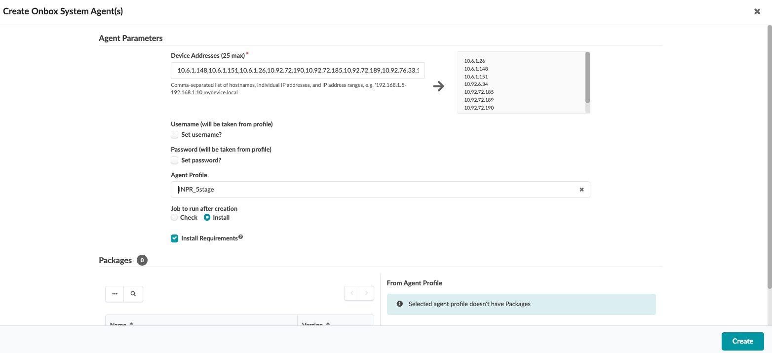
For onboarding Junos OS Evolved devices click Create Onbox agent.

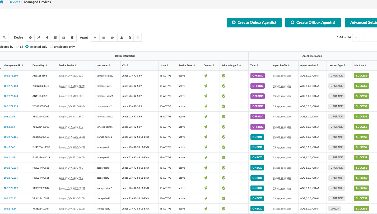
3) Apstra Web UI: Acknowledge Managed Devices for Use in Apstra Blueprints

Once the offbox and onbox agents have been added and the device information has been collected, select the checkbox interface to select all the devices and then click Acknowledge. This places the switch under the management of the Apstra server.

Finally, ensure that the pristine configuration is collected once again as Apstra adds the configurations for LLDP and RSTP.

The device state moves from OOS-QUARANTINE to OOS-READY.

Note:

Once a device is managed by Apstra, all device configuration changes should be performed using Apstra. Do not perform configuration changes on devices outside of Apstra, as Apstra may revert those changes.

Apstra Fabric Provisioning

In the following steps, the 5-stage fabric is deployed with the Juniper Apstra. Before provisioning a blueprint, a replica of the topology is created. Before datacenter Blueprint is deployed, a replica of the devices known as Logical devices and Interface Maps should be created. Logical devices are abstractions of physical devices that specify common device form factors such as the amount, speed, and roles of ports without vendor specific information. Logical devices are then mapped to the device profiles using interface maps. The ports mapped on the interface maps match the device profile and the physical device connections.

Logical devices are then used to create Racks in Apstra. Once the Racks are created the template is created for each pod which is then used to create Blueprint. For more information refer the Juniper Apstra guide to understand the terminology and device configuration lifecycle.

To create the logical devices in Apstra navigate to Design > Logical Devices

To create the Interface maps Apstra navigate to Design > Interface Maps

Apstra Web UI: Create Logical Devices, Interface Maps with Device Profiles

For the purposes of this JVD lab, logical devices and interface maps are created for all devices in Figure: 5-Stage Datacenter Architecture with Apstra.

Compute Pod logical devices and Interface maps

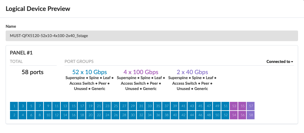
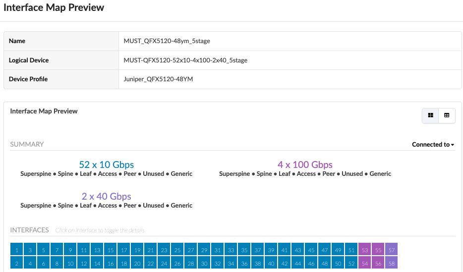
The logical devices and interface maps for QFX5120-48YM leaf switches in compute pod are shown in Figure: Logical Device for QFX5120-48YM and Figure: Interface Maps for QFX5120-48YM, the port speeds and number of ports is dependent on the setup required. The 100G ports are connections to the spine switches and the rest of the ports connect to the servers:

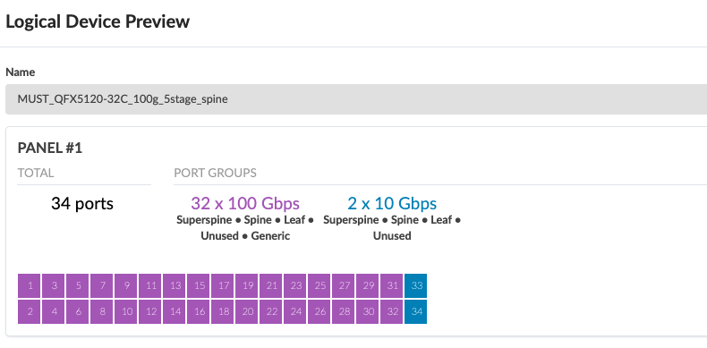
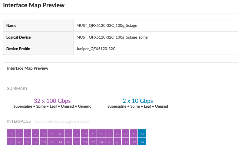
The logical devices and interface maps for QFX5120-32C Spine switches in compute pod are as below.

Storage Pod logical devices and Interface maps

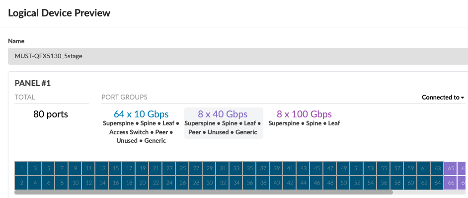
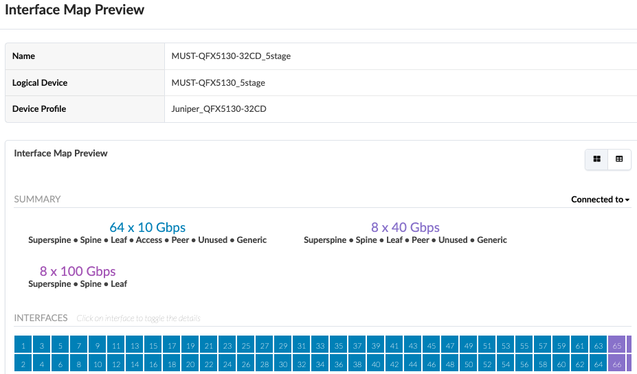
Similar to compute pod, the logical devices and interface maps for QFX5130-32CD leaf switches in storage pod are shown in Figure: Logical Device for QFX5130-32CD and Figure: Interface Map for QFX5130-32C. The 100G ports are connections to the spine switches and the rest of the ports connect to the servers.

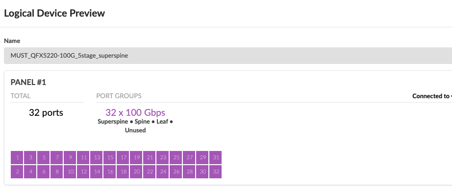
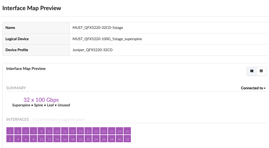
The logical devices and interface maps for QFX5220-32CD Spine switches in compute pod are as below.

Services Pod logical devices and Interface maps

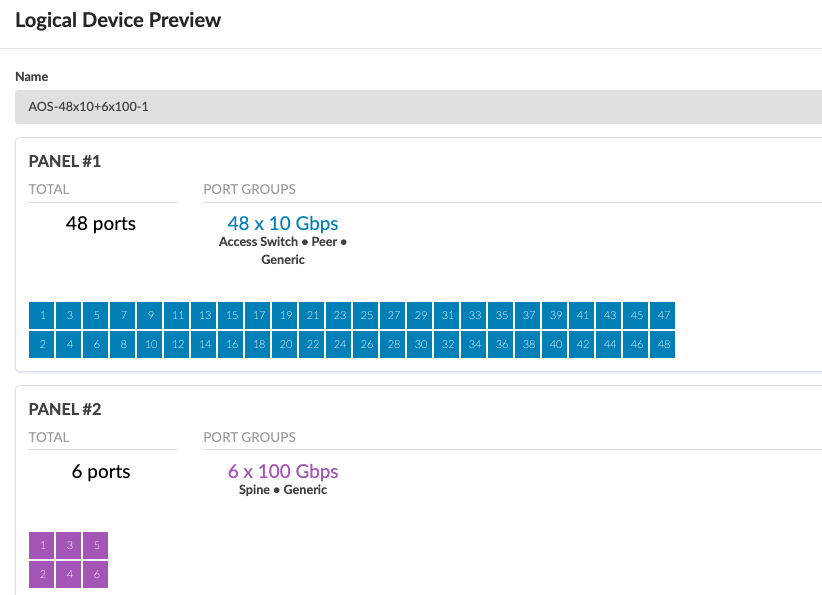
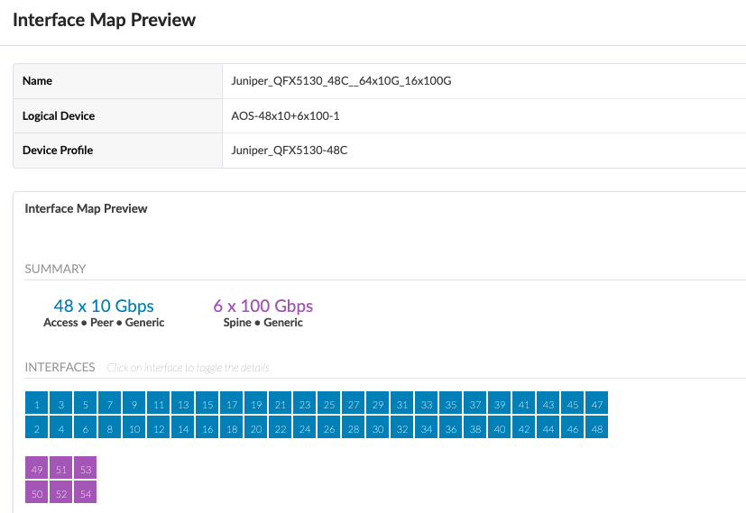
Lastly, The logical devices and interface maps for QFX5230-62CD border leaf switches in services pod are shown in Figure: Logical Device for QFX5130-48C and Figure: Interface Maps for QFX5130-48C. The 100G ports are connections to the spine switches and the rest of the ports connect to the servers.

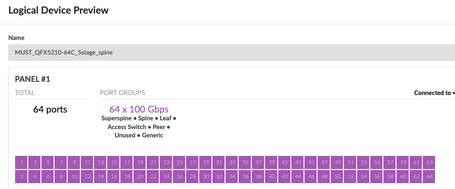
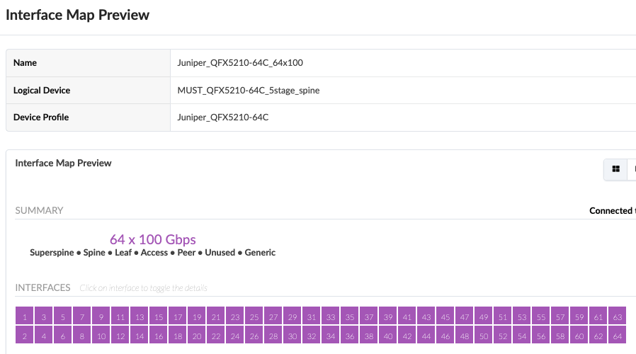
The logical device and Interface maps for the Services Pod Spine switches QFX5210-64C are as shown below.

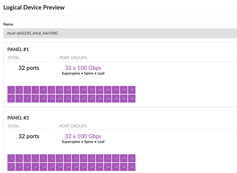
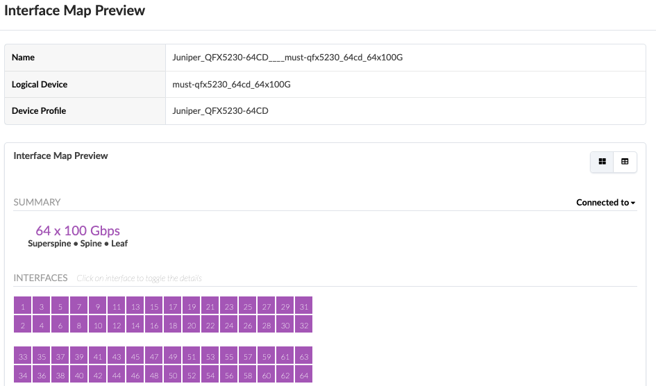
Superspine

The two superspine QFX5230-64CD connect to all the pods at the spines with 100G connection. The logical device and interface maps are shown as below in Figure: Logical device for QFX5230-64CD and Figure: Interface maps for QFX5230-64CD.

Generic servers

Apart from the above logical devices and interface maps, generic server interface maps are also required to depict the servers connected to the server leaf switches. Apstra does not manage the servers. However, generic servers define the network interface connections from the servers to the Leaf switches in respective pods.

External routers that are connected to the border leaf switches also require logical device for generic servers and corresponding interface maps. External routers used for PIM gateway and for DHCP relay from external source.

Apstra Web UI: Racks, Templates, and Blueprints—Create Racks

Once the Logical Devices and Interface Maps are created, create the necessary rack types for the 5-stage pods. For each pod a separate pod is defined as shown below.

To create Rack in Apstra, create racks under Design > Rack Types. For more information on creating racks, refer to the Juniper Apstra User Guide.

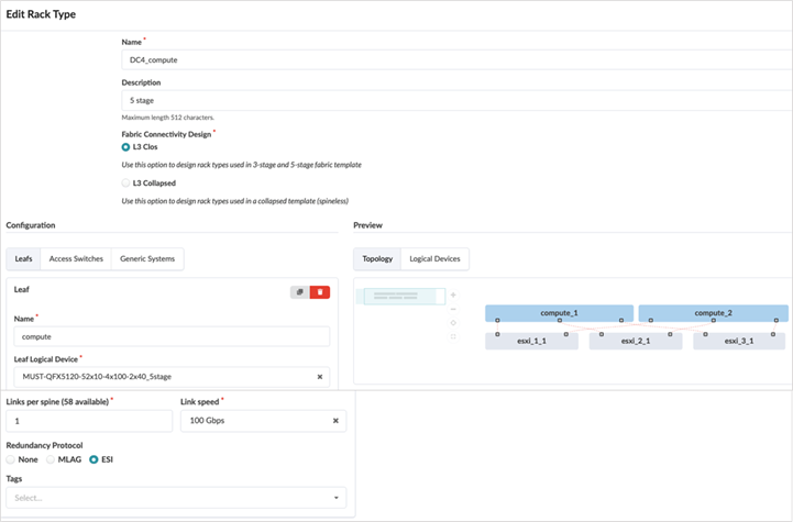
Compute Pod Rack

For the compute pod, the rack definition requires the logical device of the leaf switches as input. Generic systems define the servers and the connectivity. Along with count of systems, logical device for the servers, single-homed or dual-homed is also defined.

The services and storage pods racks are created in the same way as is created for the compute pod rack.

Templates

Once all the racks are created, a corresponding rack-based template is created in Apstra by navigating to Design > Templates > Create Template. The template defines the structure and the intent of the network. It is used to define connectivity between the ToR switches and the spine switches in the pods. This pod template is similar to 3-stage fabric datacenter design template as it consists of spine and leaf switches.

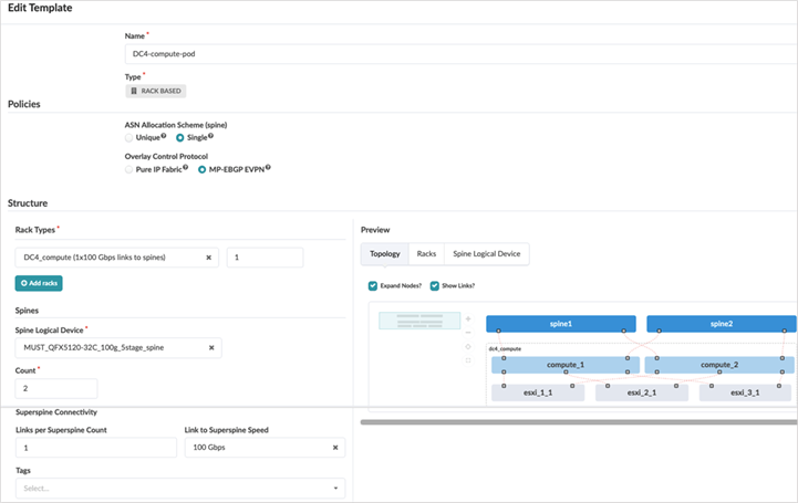
Below is screenshot of rack-based compute pod template, similar templates are created for storage and service pods. For each template the rack created in the previous step Apstra Web UI: Racks, Templates, and Blueprints—Create Racks Spine logical devices is needed along with the number count of spine switches. The connectivity to superspine should be added, as this is 5-stage rack based template, along with a count of the number of links on each superspine.

For 5-stage rack based template, choose Single ASN Allocation Schema as shown in the Figure: Compute Pod template.. All spine devices in each pod are assigned the same ASN, and all superspine devices are assigned another ASN.

And for the EVPN-VXLAN Fabric type the MP-EBGP-EVPN radio button is selected for Overlay Control Protocol.

After creating rack-based templates for each of the pods, create a pod-based template for the 5-stage Fabric. This brings all the pods together connecting them to the superspines.

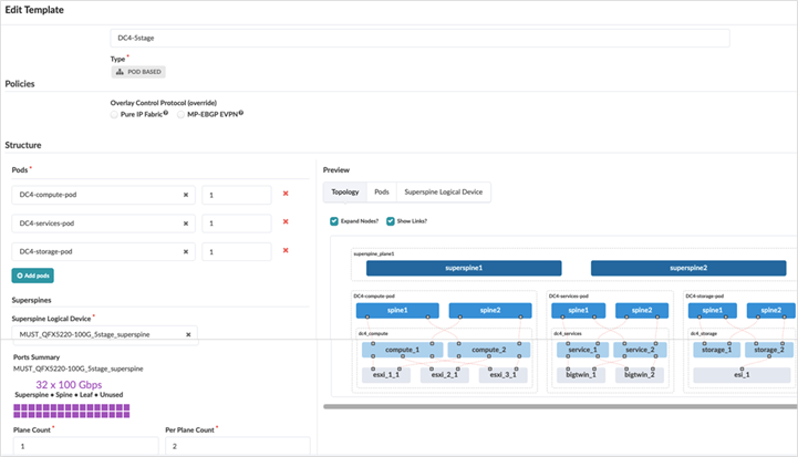
Apstra Web UI: Create a Blueprint for 5-stage Fabric

The pod-based template created in previous step above Figure: 5-Stage EVPN-VXLAN Fabric pod based Template is used as input to create Blueprint for 5-stage EVPN-VXLAN Datacenter.

To create a blueprint, click on Blueprints > Create Blueprint. For more information on creating the blueprint, see the Juniper Apstra User Guide.

It is important to select the Reference design as Datacenter and the pod-based template that was created above Figure: 5-Stage EVPN-VXLAN Fabric pod based Template IPv4 and IPv6 dual stack is selected for fabric underlay and overlay links.

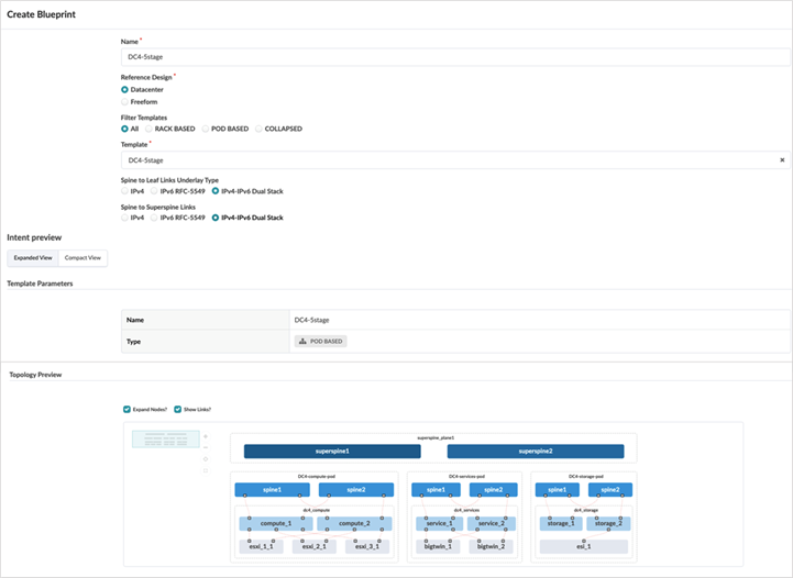
Once the blueprint is created, it’s ready for assigning resources, mapping interface maps, and assigning devices to the fabric switch roles. The blueprint is created as shown below.

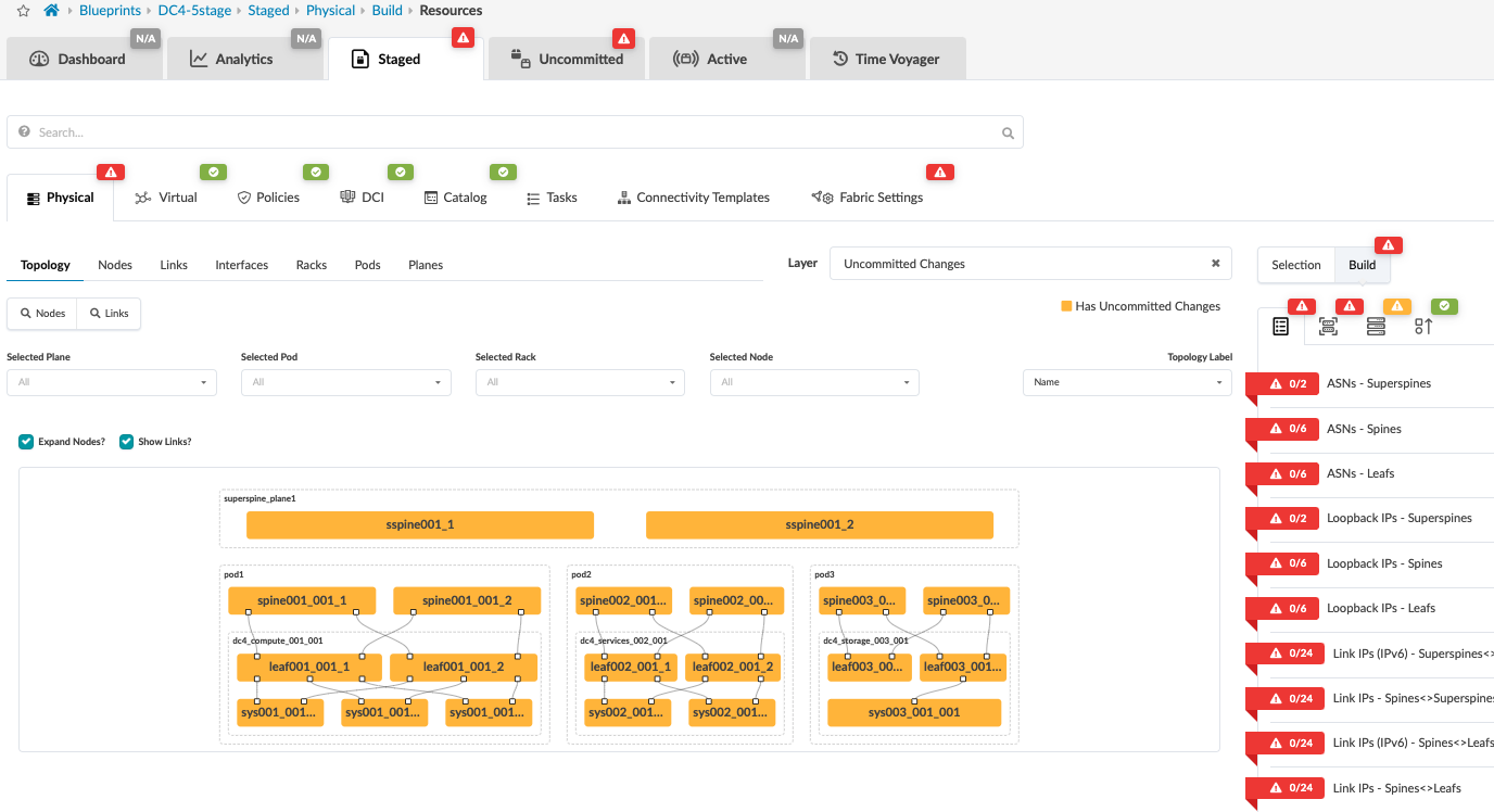
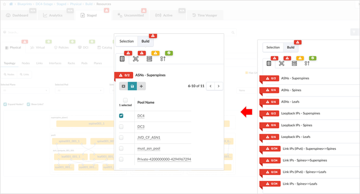
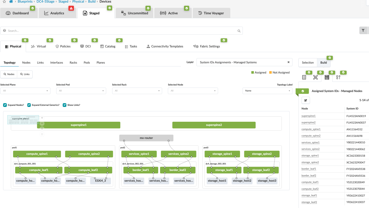
Assign Resources

In this step, the resources are allocated using the pools created in Apstra under Resources. Resources such as ASN, Loopback IP, Fabric Link IPs can be created and used and assigned to superspines, spines, leaf switches.

Assign Interface Maps and devices

The next step is to assign Interface maps for each switch’s role. This allows Apstra to map the interfaces on devices (using device profile) with the actual device once the devices are assigned to their roles.

Note:

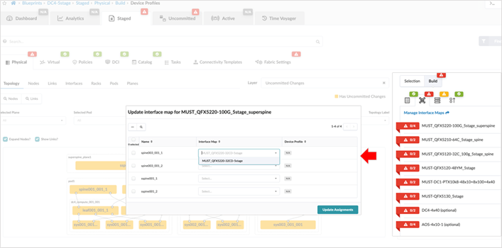
While assigning devices to the role, in case a device serial number is not visible then navigate to Devices > Managed Devices and verify that the device that was being assigned has the right device profile and corresponding Interface map.

Review Cabling

Apstra automatically assigns cabling ports on devices that may not be the same as the physical cabling. However, the cabling assigned by Apstra can be overridden and changed to depict the actual cabling. This can be achieved by accessing the blueprint, navigating to Staged > Physical > Links, and clicking the Edit Cabling Map button or use the Fetch discovered LLDP data. For more information, refer to the Juniper Apstra User Guide.

Apstra Web UI: Creating Configlets in Apstra

Configlets are configuration templates defined in the global catalog under Design > Configlets. Configlets are not managed by Apstra’s intent-based functionality, and should be managed manually. For more information on when not to use configlet refer to the Juniper Apstra User Guide. Configlets should not be used to replace reference design configurations. Configlets can be declared as a Jinja template of the configuration snippet, such as Junos configuration JSON style or Junos set-based configuration.

Note:

Improperly configured configlets may not raise warnings or restrictions. It is recommended that configlets are tested and validated on a separate dedicated service to ensure that the configlet performs exactly as intended. Passwords and other secret keys are not encrypted in configlets.

Property sets are data sets that define device properties. They work in conjunction with configlets and analytics probes. Property sets are defined in the global catalog under Design > Property Sets.

Configlets and property sets defined in the global catalogue need to be imported into the required blueprint and if the configlet is modified then the same needs to be reimported into the blueprint, as is the case with property sets too. The following figure shows configlets and property sets located on a blueprint.

During 5-stage validation, several configlets were applied either as part of the general configuration for setup and management purposes (such as nameservers, NTP, and so on). Since Apstra 5.0 doesn’t support OISM, ECN and PFC configuration using QOS, loopback firewall policies and firewall policies, configlets are used to configure those settings. This will be covered separately.

Fabric Setting

This option allows for fabric-wide setting of various parameters such as MTU, IPv6 application support, and route options. For this JVD, the following parameters were used: View and modify these settings within the blueprint Staged > Fabric Settings > Fabric Policy within the Apstra UI.

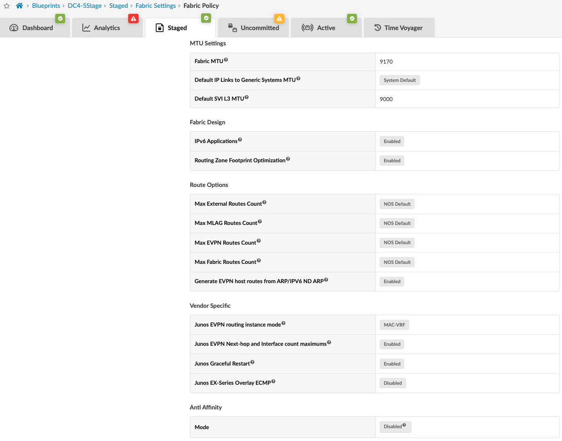
To simulate moderate traffic in datacenter, traffic scale testing was performed. Refer to Table: Scaling Numbers Tested for more details. The scale testing was performed on switches.

The setting Junos EVPN Next-hop and Interface count maximums was also enabled. This allows Apstra to apply the relevant configuration to optimize the maximum number of allowed EVPN overlay next-hops and physical interfaces on leaf switches to an appropriate number for the data center fabric.

For more information on these features, refer to:

https://www.juniper.net/documentation/us/en/software/junos/multicast-l2/topics/topic-map/layer-2-forwarding-tables.html

https://www.juniper.net/documentation/us/en/software/junos/cli-reference/topics/ref/statement/next-hop-edit-forwarding-options-vxlan-routing.html

For the Junos EVO devices, following host-profile setting was configured on the Junos EVO switches to allocate memory based on higher mac scale.

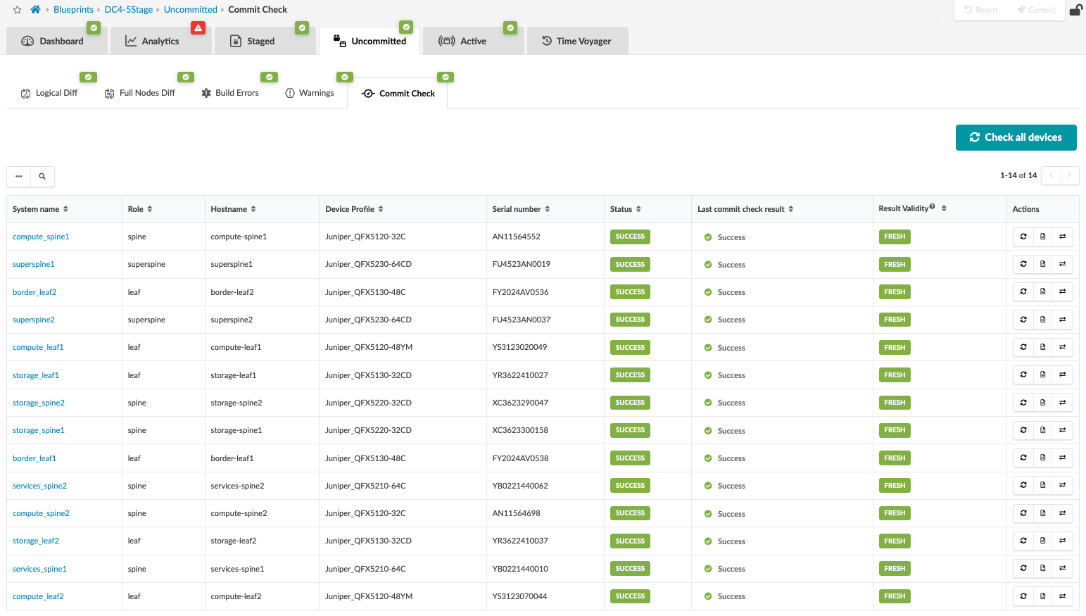
Commit Configuration

Once all the above steps are completed, the fabric is ready to be committed. This means that the control plane is set up, and all the leaf switches are able to advertise routes through BGP. Review changes and commit by navigating from the blueprint to Blueprint > <Blueprint-name> Uncommitted.

Starting with Apstra 4.2, a new feature to perform a commit check before committing, was introduced to check for semantic errors or omissions, especially if any configlets are involved.

Note that if there are build errors, those need to be fixed. Otherwise, Apstra will not commit any changes until the errors are resolved.

For more information, refer to the Juniper Apstra User Guide.

The blueprint for the data center should indicate that no anomalies are present to show that everything is working. To view any anomalies with respect to blueprint deployment, navigate to Blueprint > <Blueprint-name> > Active to view the anomalies raised with respect to BGP, cabling, interface down events, routes missing, and so on. For more information, refer to the Apstra User Guide.

Overlay network with Virtual Network and Routing Zone can now be provisioned. For more information on provisioning overlay network refer the Juniper Apstra User guide.

Configuring Optimized Intersubnet Multicast (OISM)

Optimized intersubnet multicast (OISM) is a multicast traffic optimization feature that operates at L2 and L3 in EVPN-VXLAN edge-routed bridging (ERB) overlay fabrics. OISM uses the concept called Supplemental Bridge Domain (SBD) to optimize scaling in the fabric. The SBD is configured on leaf devices and hence the remote tenant bridge domains are reachable via SBD. This simplifies the implementation of OISM in an ERB architecture datacenter design. OISM employs an SBD inside the fabric as follows:

• The SBD has a different VLAN ID from any of the revenue VLANs.
• Border leaf devices use the SBD to carry the traffic from external sources toward receivers within the EVPN fabric.
• In enhanced OISM mode, server leaf devices use the SBD to carry traffic from internal sources to other server leaf devices in the EVPN fabric that are not multihoming peers.

In EVPN ERB overlay fabric designs, the leaf switches in the fabric route traffic between tenant bridge domains. When OISM is enabled, the leaf devices selectively forward traffic to leaf devices with interested receivers. This improves traffic performance within the EVPN fabric. ERB overlay fabrics can efficiently and effectively support multicast traffic flow between devices inside and outside the EVPN fabric. OISM optimizes the number of next-hop flooding only to the leaf switches.

OISM also supports other protocols such as Internet Group Management Protocol (IGMP) snooping and Multicast Listener Discovery (MLD) snooping. These protocols constrain multicast traffic in a broadcast domain to interested receivers and multicast devices, therefore preserving bandwidth. For external sources and receivers, PIM gateways at border leaves enable the exchange of Multicast traffic between internal sources and receivers and external sources and receivers.

The border leaves can connect to the external PIM router using any of the methods provided below to exchange multicast traffic:

• M-VLAN IRB method: A dedicated VLAN called M-VLAN and IRB interface is used to only exchange traffic flow to and from the external PIM domain. The M-VLAN IRB interfaces is used to extend in the EVPN instance.

Note:

M-VLAN method is not supported on enhanced OISM.

• Classic L3 interface method: Classic physical L3 interfaces on OISM border leaf devices connect individually to the external PIM domain on different subnets. There is no VLAN associated with these interfaces.
• Non-EVPN IRB method: A unique extra VLAN ID and subnet for the associated IRB interface is assigned to IRB interfaces on border leaves. This IRB interface is not extended in the EVPN instance.

For more information on OISM refer this OISM guide.

For the purposes of this JVD, OISM with Bridge Domain Not Everywhere (BDNE) (also known as enhanced OISM) is configured across all the leaf switches mentioned in Table: Devices under Test connecting to sources and receivers. This means that the revenue bridge domains need not be configured on all the leaf switches.

Configuration for enhanced OISM:

In enhanced OISM (BDNE), enhanced-OISM statement is configured across all leaf switches including border leaf switches under [edit forwarding-options multicast-replication evpn irb].

Since OISM is not supported in Apstra version 5.0, configlets are used to configure the server leaf switches and border leaf switches. OISM requires OSPF to exchange traffic routes. For enhanced OISM, OSPF is configured on all leaf switches on the SBD IRB interface in each tenant VRF instance.

Server leaf switch config

Compute leaf switches

The enhanced-oism option is enabled. The supplemental bridge domain is configured with VLAN 3500 as shown in config snippet. The server leaf device is configured to accept multicast traffic from the SBD IRB interface as the source interface using the accept-remote-source statement at the [edit routing-instances name protocols pim interface irb-interface-name] hierarchy level. PIM protocol is also configured as passive on all leaf switches. IGMP is also configured to exchange multicast traffic to interested receivers. OSPF is configured at [edit routing-instances name protocols OSPF] hierarchy level . The SBD IRB interface (irb.3500) and loopback interface are configured as active mode. All other interfaces are configured as passive mode.

Note:

Ensure the MTU on the SBD IRB interface is lower than the IRB MTUset protocols igmp interface all

Storage Leaf switches

The conserve-mcast-routes-in-pfe option is required to be configured for QFX5130-32CD if used as server leaf or border leaf. With this option, the QFX5130-32CD switches conserve PFE table space by installing only the L3 multicast routes and avoid installing L2 multicast snooping routes. This option is set in all OISM-enabled MAC-VRF EVPN routing instances on the device.

The rest of the configuration is same as compute pod leaf switches.

Note:

The conserve-mcast-routes-in-pfe should be deleted if OISM is disabled.

Border Leaf switches

The border leaf switches act as PIM EVPN gateway (PEG) interconnecting the EVPN fabric to multicast devices (sources and receivers) outside the fabric in an external PIM domain. In this case, the border leaf switches connect to the external PIM router using Classic L3 method.

The configuration option pim-evpn-gateway is configured under [edit routing-instances blue protocols evpn oism].

The revenue bridge domain 1400 and 1401 are configured as distributed-DR and the SBD 3500 is configured as standard mode at the [edit routing-instances name protocols pim interface irb-interface-name] hierarchy level.

The connectivity between border leaf switches and the external PIM router is using Classic L3 method. The PIM router acts as PIM rendezvous point (RP). Lastly OSPF is configured at [edit routing-instances name protocols OSPF] hierarchy level to learn routes to multicast sources to forward traffic from external sources toward internal receivers, and from internal sources toward external receivers. The SBD IRB interface and the external multicast L3 interface are configured as PIM active mode. All other interfaces are configured as passive mode.

Connection to external PIM router

Note:

Apstra does not support OSPF natively. Hence it is recommended to use the custom telemetry, collector and probes as discussed in Apstra UI: Blueprint Dashboard, Analytics, probes, Anomalies.

Apstra UI: Blueprint Dashboard, Analytics, probes, Anomalies

Apstra provides predefined dashboards that collect data from devices. With the help of Intent-Based Analytics (IBA) probes, Apstra combines intent with data to provide real-time insight into the network, which can be inspected using Apstra GUI or Rest API. The IBA probes can be configured to raise anomalies based on the thresholds.

Custom Telemetry and Probes

From Apstra 4.2 onwards, custom telemetry collectors can be created to monitor data which Apstra can use for analyzing. With the custom telemetry collection, the following can be achieved:

• Run Junos CLI show commands that provides data for analyzing.
• Identify the specific key and value to extract from the show command based on its XML output.
• Create a telemetry collector definition.
• Create an IBA probe that utilizes the data from the telemetry collector.

The Apstra guide walks through the steps for setting up custom telemetry collector and custom probes.

Apstra also provides some example custom collector and probes which can be customized as is required. The GitHub link is as below.

https://github.com/Juniper-SE/Apstra_IBA_Probes.git

Congestion Management with RDMA Over Converged Ethernet v2 (ROCEv2)

The 5-stage datacenter design is based on a compute, storage and services (web) pod design which means the fabric should be able to handle moderate to very high amount of storage traffic reliably within the fabric.

Data Center Quantized Congestion Notification (DCQCN), has become the industry-standard for end-to-end congestion control for RDMA over Converged Ethernet (RoCEv2) traffic. DCQCN congestion control methods offer techniques to strike a balance between reducing traffic rates and stopping traffic all together to alleviate congestion, without resorting to packet drops.

DCQCN combines two different mechanisms for flow and congestion control:

• Priority-Based Flow Control (PFC), and
• Explicit Congestion Notification (ECN).

Priority-Based Flow Control (PFC) helps relieve congestion by halting traffic flow for individual traffic priorities (IEEE 802.1p or DSCP markings) that are mapped to specific queues or ports. The goal of PFC is to stop a neighbor from sending traffic for a period of time (PAUSE time), or until the congestion clears. This process consists of sending PAUSE control frames upstream requesting the sender to halt transmission of all traffic for a specific class or priority while congestion is ongoing. The sender completely stops sending traffic to the requesting device for the specific priority.

While PFC mitigates data loss and allows the receiver to catch up processing packets already in the queue, it impacts performance of applications using the assigned queues during the congestion period. Additionally, resuming traffic transmission post-congestion often triggers a surge, potentially exacerbating or reinstating the congestion scenario.

Explicit Congestion Notification (ECN), on the other hand, curtails transmit rates during congestion while enabling traffic to persist, albeit at reduced rates, until congestion subsides. The goal of ECN is to reduce packet loss and delay by making the traffic source decrease the transmission rate until the congestion clears. This process entails marking packets with ECN bits at congestion points by setting the ECN bits to 11 in the IP header. The presence of this ECN marking prompts receivers to generate Congestion Notification Packets (CNPs) sent back to source, which signal the source to throttle traffic rates.

Combining PFC and ECN offers the most effective congestion relief in a lossless fabric supporting RoCEv2, while safeguarding against packet loss. To achieve this, when implementing PFC and ECN together, their parameters should be carefully selected so that ECN is triggered before PFC. The fill level and the drop-probability are the most important parameters to manage traffic during congestion. Here is a sample config for setting these parameters.

Note:

Note that these may vary for each datacentre, so its recommended to test this before implementing.

For more information on the congestion management, refer the document for Congestion management in Juniper AI/ML Networks

In this 5-stage JVD, the leaf switches were configured with class of service using configlet. The configs can be viewed on github link.