
Add a Graph Query
Next, we need to add a graph query to the new probe. Before starting, review the graph database overview explained in the following section. Otherwise, to continue with the configuration, proceed to Add Graph Queries to the Probe.
Graph Database Overview
The Apstra graph database is an in-memory, distributed datastore (DDS). It models network intent as interconnected nodes, including switches, interfaces, links, services, policies, and routing zones, with directed relationships that show connections and dependencies.
Role of a Graphy Query in IBA
A graph query in a source processor defines the scope of telemetry collection. This scoping is enforced by mapping graph query results to telemetric keys, such as IP addresses. In our case, the telemetry service key is an IP address, so the query must obtain IP addresses. There are three BGP sessions: Underlay, Overlay, and External BGP Sessions. Let’s examine graph queries for all BGP sessions.
Before exploring graph queries, we must first understand static and dynamic series graphs in IBA.
-
Static series (graph-driven)
The graph scope determines the set of series. Graph query results control the data fed into the probe by the service collector. Mapping query results to telemetry service keys, defined in the service schema, achieves this. These series are called "static" because they stay unchanged unless the graph changes.
-
Dynamic series (collector-driven)
Dynamic series graphs respond to switch conditions, regardless of graph state. The telemetry service on the device defines the series dynamically. The graph specifies which systems execute the service but omits key service aspects.
This approach is useful for monitoring components absent in the graph database, including:
-
Power supplies
-
Optical transceivers
-
Configuration elements without graph properties
These series are called "Dynamic" because they respond to switch activity independently of the graph state.
-
Graph Query Examples
This section includes three graph queries we'll use to determine the Remote IP Address of the BGP Protocol running for Underlay, Overlay, and External BGP sessions.
Underlay BGP Graph Query
A blueprint includes interfaces connecting to generic systems, external routers, and the fabric side. In this setup, the first BGP sessions act as Underlay sessions. Apstra’s Reference Design specifies that Underlay BGP sessions are established on physical interfaces facing the fabric. The graph query retrieves IPv4 addresses for all fabric-facing links and interfaces.
Example: Graph Query for Underlay BGP Sessions
match(
  node('system', name='system', deploy_mode='deploy', role=is_in(['leaf', 'spine']))
    .out('hosted_interfaces')
    .node('interface', name='iface', if_name=not_none())
    .out('link')
    .node('link', link_type='ethernet', name='link', role='spine_leaf')
    .in_('link')
    .node('interface', name='remote_iface')
    .in_('hosted_interfaces')
    .node('system', role=is_in(['spine', 'leaf', 'superspine']), deploy_mode='deploy',
name='remote_system')
)
  .ensure_different('system', 'remote_system')
Overlay BGP Graph Query
Overlay BGP connects over loopback interfaces, specifically Loopback0
(lo0) per Apstra's Design Reference. End-to-end overlay
BGP sessions link leaf devices. The graph query must retrieve loopback IPs
for all leaf devices with overlay BGP sessions. The lo0
interface acts as a logical interface within the device.
Example: Graph Query for Overlay BGP Sessions
match(
  node('system', name='system', deploy_mode='deploy', role=is_in(['leaf', 'spine']))
    .out('hosted_interfaces')
    .node('interface')
    .out('link')
    .node('link', name='link')
    .in_('link')
    .node('interface')
    .in_('hosted_interfaces')
    .node('system', role=is_in(['leaf', 'spine']), deploy_mode='deploy', name='remote_system')
    .out('hosted_interfaces')
    .node('interface', if_type='loopback', loopback_id=0, name='remote_iface'),
  node(name='system')
    .out('hosted_interfaces')
    .node('interface', loopback_id=0, name='iface')
)
  .ensure_different('system', 'remote_system')
  .distinct(['system', 'remote_system', 'remote_iface'])
External BGP Graph Query
External BGP sessions run on physical interfaces connected to external routers or generic systems, not fabric-facing ports. According to the Apstra Reference Design, these ports connect to external routers or generic systems. External BGP sessions are configured for the default BGP table and routing-instances table in this setup.
The graph query must return the IP address of all system-facing links from the leaf where:
-
BFD is enabled.
-
The link is a protocol endpoint.
-
The interface type is a sub-interface.
Example: Graph Query for External BGP Sessions
match(
  node(name='iface', type=is_in(['interface', 'ip_endpoint']), if_type="subinterface")
    .in_('layered_over')
    .node('protocol_endpoint')
    .in_('instantiates')
    .node('protocol_session', bfd=True)
    .out('instantiates')
    .node('protocol_endpoint')
    .out('layered_over')
    .node('interface', name='remote_iface')
    .ensure_different('iface', 'remote_iface'),
  node(name='iface', if_type="subinterface")
    .in_('composed_of')
    .node('interface')
    .in_('hosted_interfaces')
    .node('system', name='system', role="leaf"),
  node(name='remote_iface')
    .out('link')
    .node('link', name='link')
)
Add Graph Queries to the Probe
To add the graph queries:
-
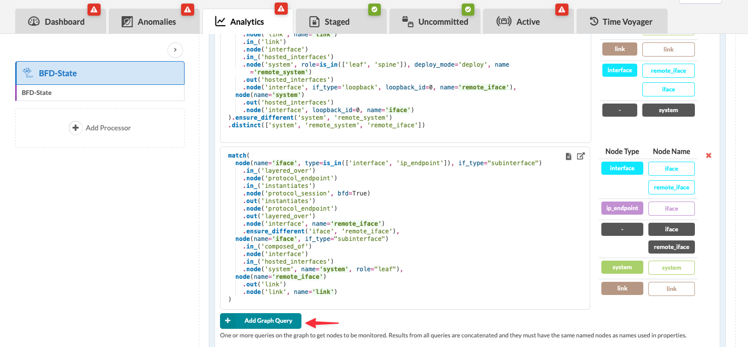
Add all three graph queries to the BFD-State source
processor (Extensible Service Collector) as shown in Graph Query Examples.
Click Add Graph Query for each query twice to open three queries. Then paste the examples into all three queries.
-
Define the Telemetry Data.
Graph queries inform the processor about the systems needed to run the service. Define the following parameters in the telemetry section of the source processor BFD_States to enable the service:
Table 1: Telemetry Settings Setting Description System ID system.system_idService name Specify the service name defined in the previous section. In this case, use BFD_Session_Check. Service interval Telemetry collection interval. Determines how frequently the service collects data. Key Name and Value Retrieves the key defined within in the service, specifically "Remote IP,"and maps it to a graph expression. The system assigns the value as str(remote_iface.ipv4_addr.split('/')[0]).The graph database uses the "IP address/subnet mask" format. The telemetry service uses the "IP address" format.
The expression breakdown is:
-
remote_iface.ipv4_addr: retrieves the IPv4 address attribute, which typically includes a value like192.168.1.0/24. -
.split('/'): divides the string at the forward slash character, creating a list with two elements:192.168.1.0,24 -
[0]: selects the first element from the resulting list, which is the IP address excluding the subnet mask.
Data Type Map keys and values in the service collector. We chose Static series because it is graph-driven and maps keys and values through restricted collected data. 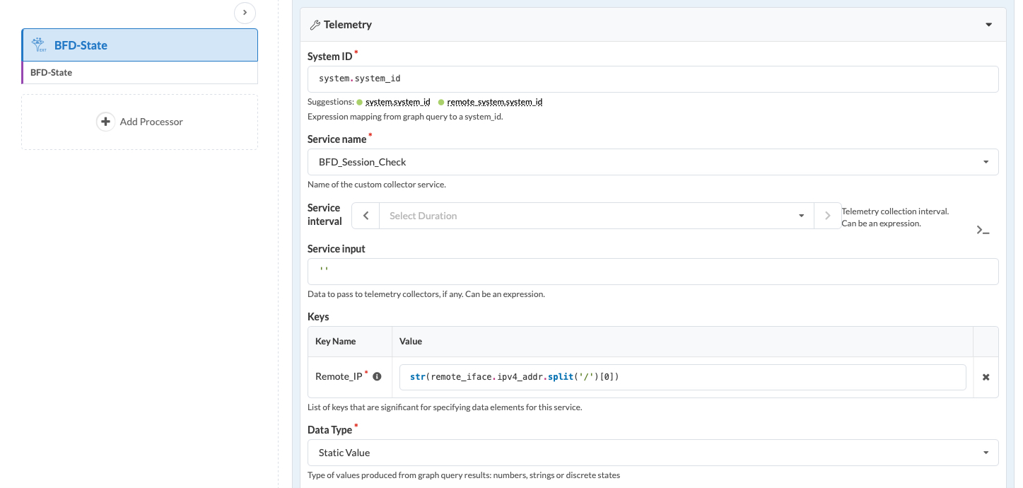
-
-
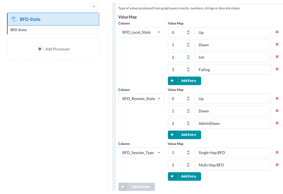
Enter the Value Map values.
Value Map maps discrete-state values to human-readable strings for all applicable output columns. The Select Node section explains how expression-based mapping converts BFD local and remote states, and session type, from strings to sequences of integer values.
IBA processes these values as discrete states and converts them back to their corresponding BFD States and session-type values. The Select Node emphasizes that the sequence matters, not the number. This is crucial for handling these values as discrete in IBA.
To enter the value map values:
-
Click Add Column. The drop-down menu lists
all discrete values. Make sure you select one value at a time. To
add multiple values, click Add Entry.
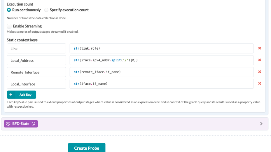
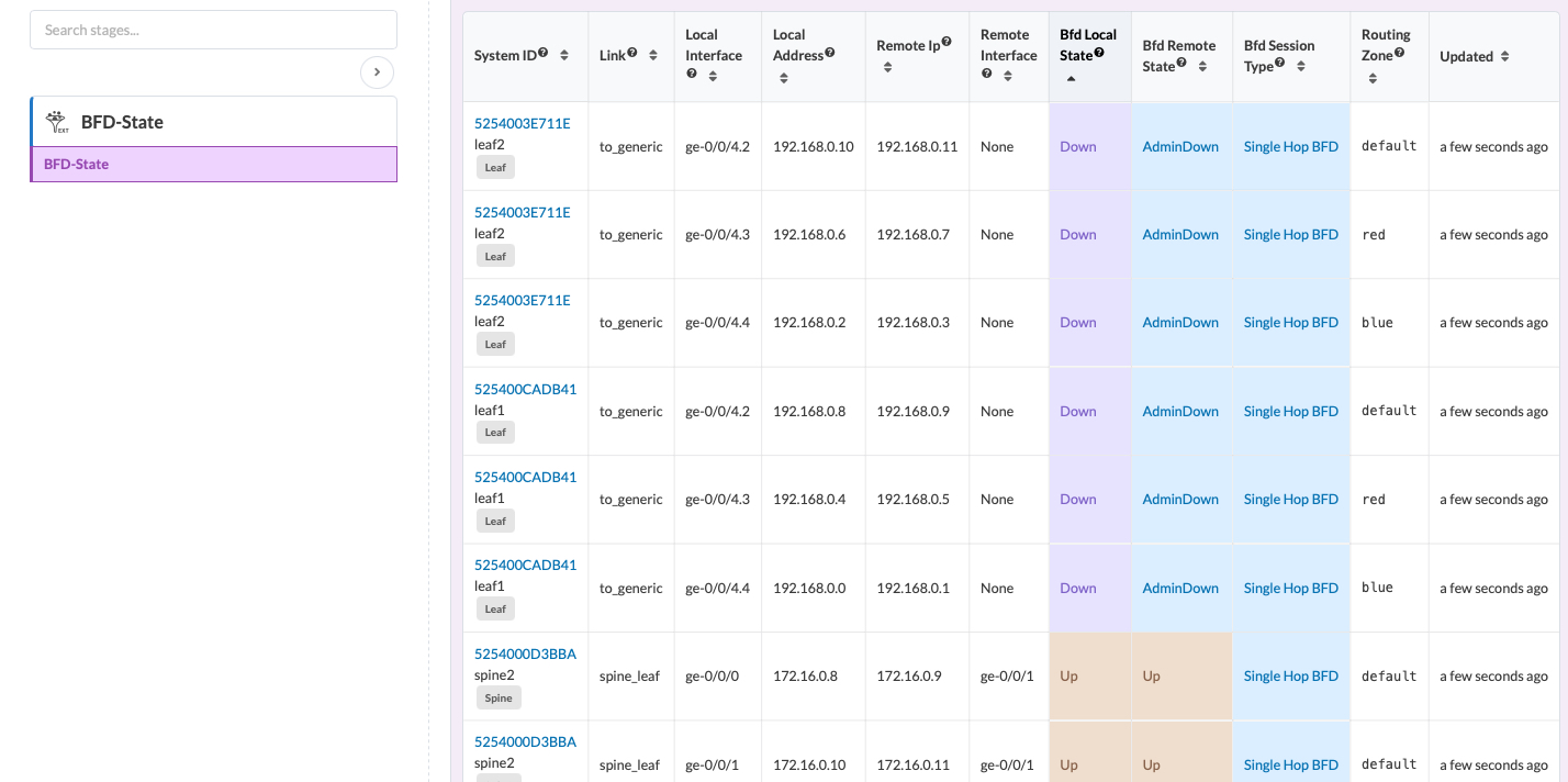
Use static context keys to add properties to the processor’s output. Each key represents a property name with a value evaluated in the graph query context. The processor writes the results under the key in the output.
-
Key: Name of the property to add.
-
Value: An expression that runs in the graph context; its result becomes the property key(s) value. The expression to define this value is
node.attribute.
Refer to the following table for descriptions of property keys and their values used in this setup.
Table 2: Property Key and Value Descriptions Property Key Value Link Use this property to add output from one of the attributes of the linknode from the graph query.The
roleattribute provides information about the role of a particular link between two devices in string output, such asspine_leaforto_generic.Define this value with the expression
link.role.Local_Address Use this property to add the output from one of the attributes of the ifacenode from the graph query.The
ipv4_addrattribute provides information about the IPv4 address configured on that respective port. This attribute returns an IPv4 address in IPv4/subnet format (CIDR format).To extract only the IPv4 address, use the expression
str(iface.ipv4_addr.split('/')[0]). Usesplit('/')[0]to remove the subnet portion from the value and return only the IPV4 address in the outputRemote_Interface Use this property to add the output from one of the attributes of the remote_ifacenode from the graph query.The attribute isif_name, which provides information about the remote interface—for example, ge-0/0/1, xe-1/0/0, and so on.Define this value with the expression
remote_iface.if_name.Local_Interface Use this property to add the output from one of the attributes of the ifacenode from the graph query. The attribute isif_name, which returns the local interface name, such as ge-0/0/2 and xe-1/1/0.Use the expression
iface.if_nameto return this value.Static Context Keys Enter these values for static context keys: - Link:
str(link.role) -
Local Address:
str(iface.ipv4_addr.split('/')[0]) - Remote_Interface:
str(remote_iface.if_name) - Local_Interface:
str(iface.if_name)
-
-
Click Add Column. The drop-down menu lists
all discrete values. Make sure you select one value at a time. To
add multiple values, click Add Entry.
-
Select Add Key under
Advanced. Then enter the static key name and
values, and select Create Probe.
Next, continue to Add an Analytical Processor.