
Configure a Custom Telemetry Service
This topic describes the steps for configuring a customized telemetry service with the XML Transform node, Join node, Select node, and Service Sink node, using BFD-related metrics as an example.
Add an XML Transform Node
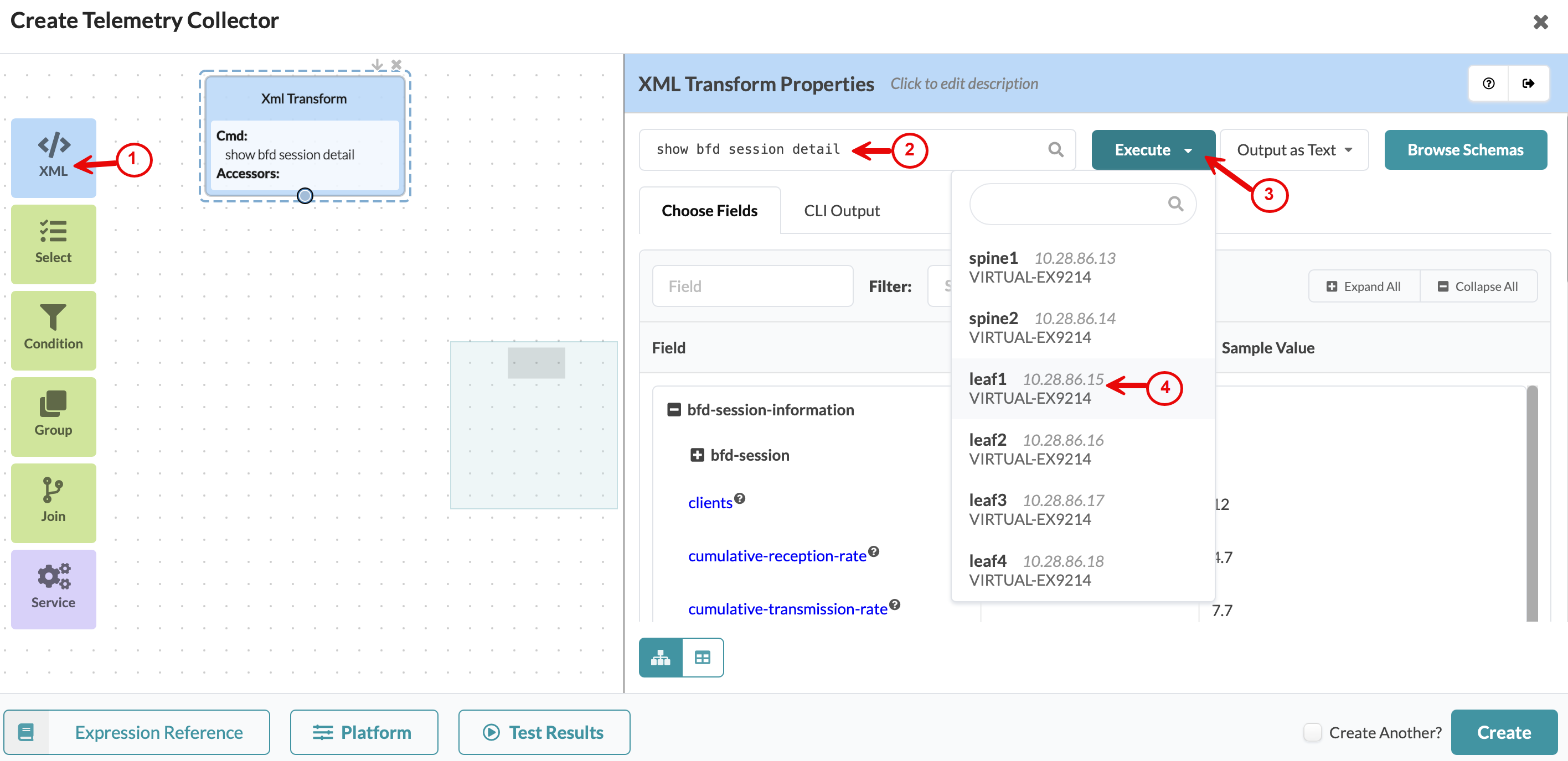
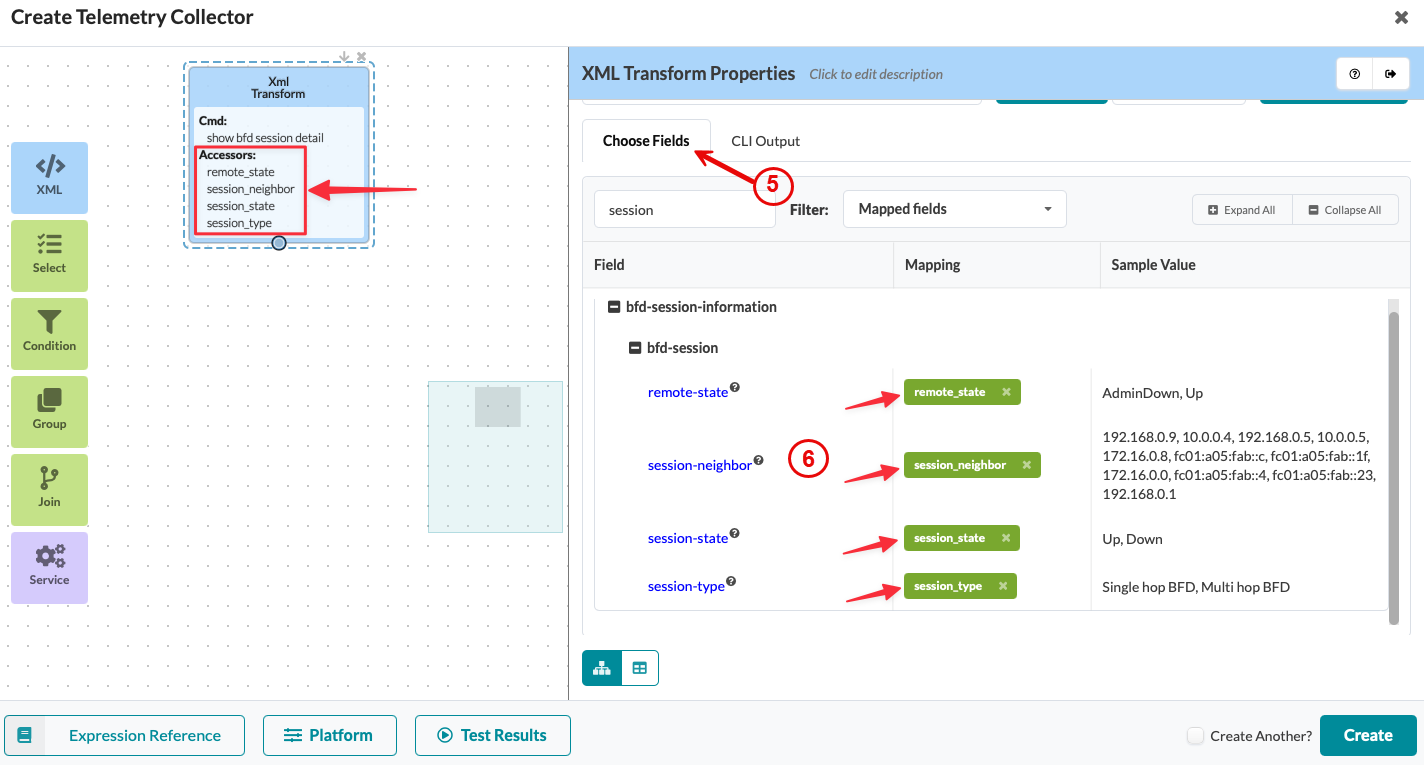
A collector pipeline always starts from an XML Transform node, which defines data ingestion. This node specifies the CLI command and defines the parsing logic. The accessor definition extracts the fields of interest from the CLI command output text.
To add an XML Transform node:
-
Select the XML icon on the Create
Telemetry Collector page.
-
Click the Choose Fields tab.
-
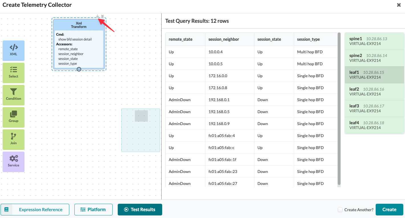
Click Run up to this node—an arrow on top of the
node—to test the results. This output displays all field-value pairs for the
BFD protocol. This step lets you verify the node test results.The output
displays all field and value pairs for the BFD protocol.
The Test Query Results table in the image below shows the results for the ingested data accessors. The BFD protocol output includes all field-value pairs and shows a typical collector output with mixed IPv4 and IPv6 sessions. This example monitors BFD exclusively for IPv4 sessions, excluding IPv6 sessions.
-
Add a second XML Transform node to process BGP CLI data. Adding the second
node is necessary because the BFD CLI output does not include all required
BGP session details.
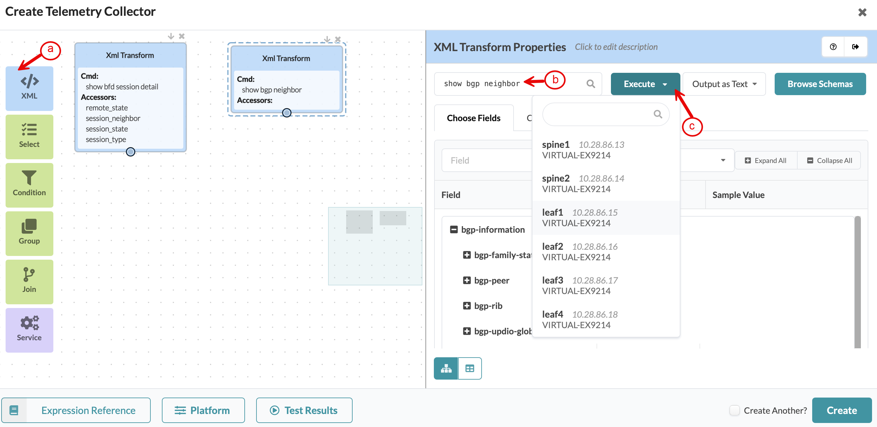
To add a second XML Transform node:
-
Select the accessors for the second node. For BGP, we selected the
following:
-
local-address -
peer-address -
table-name -
address-families
The second XML Transform node extracts all specified mapped fields from the list of accessors and displays the following fields: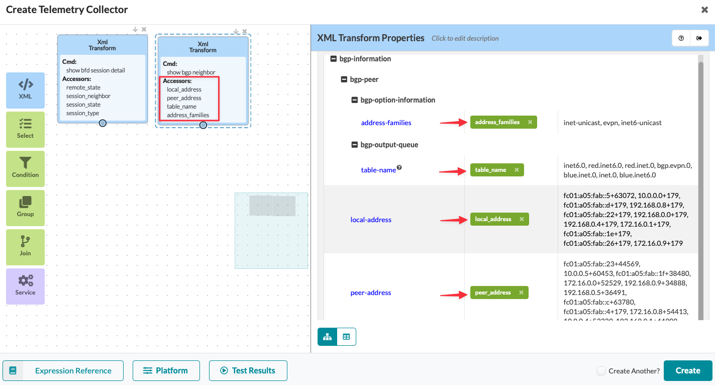
-
-
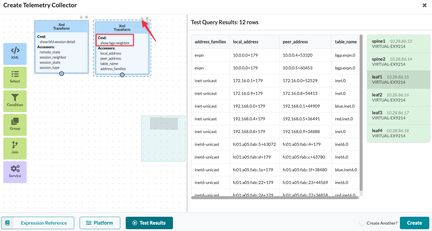
Click Run up to this node—an arrow on top of
the node— to test the results of the second XML Transform
node.
-
Select the accessors for the second node. For BGP, we selected the
following:
Merge the Ingested Data Using the Join Node
To merge the ingested data using the Join node:
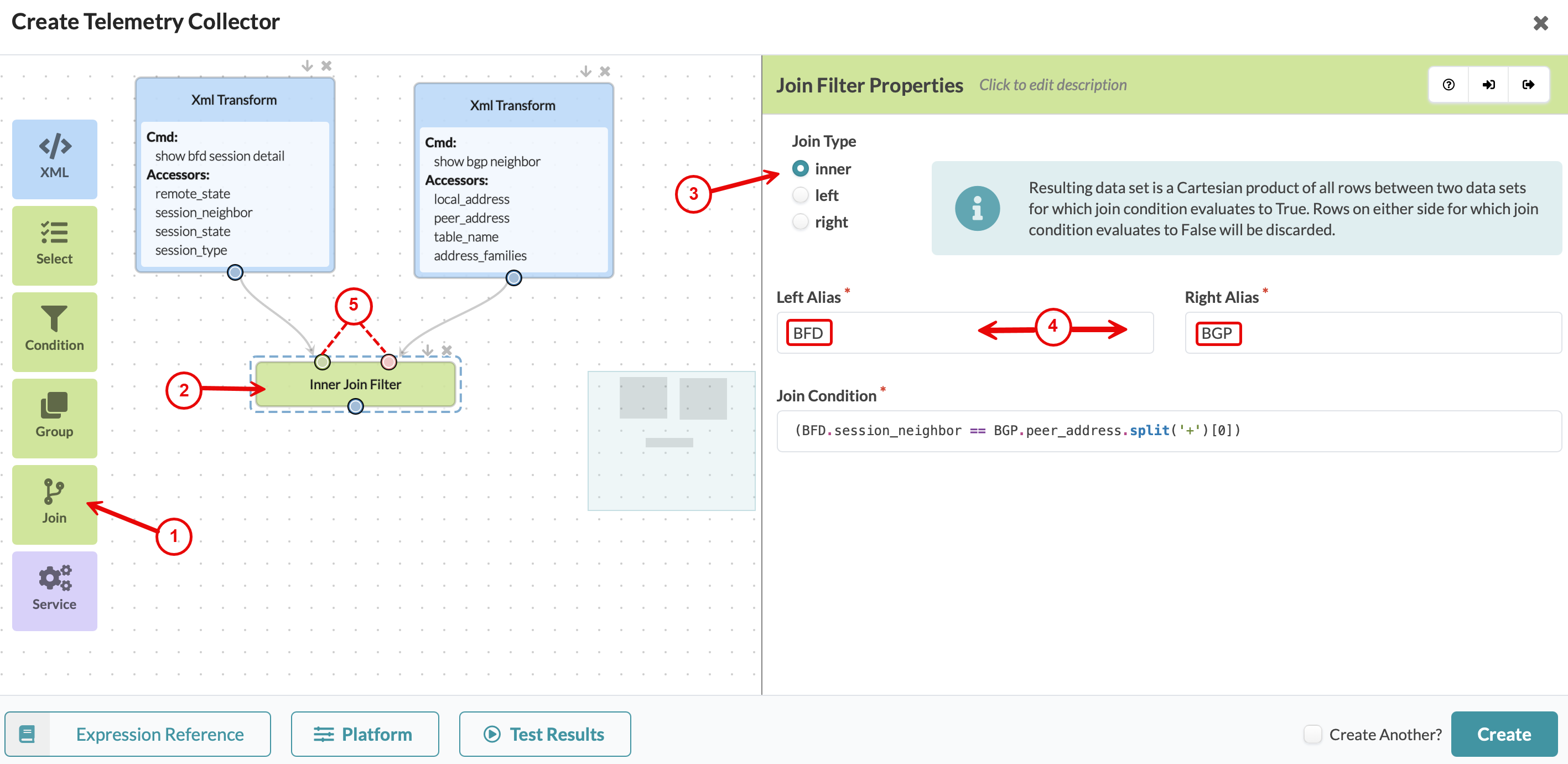
-
Select the Join icon on the Create
Telemetry Collector page.
-
Test the results of the Join node by clicking the
down arrow on the Inner Join Filter
The following image displays the query results and verifies that the BFD
session_neighborand BGPpeer_addressvalues match. You can also view other fields ingested through this node across all 12 rows, each representing a single session.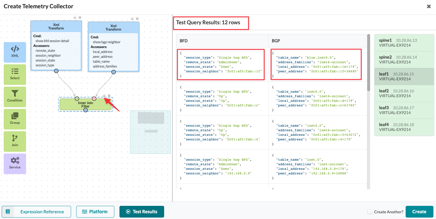
Define the Service Output Using the Select Filter Node
The Select Filter node is a data transformation component that processes input data by applying expression-driven transformations to generate a modified output. The node's primary purpose is to restructure data into a format acceptable to the telemetry service, resulting in producing the service's schema.
A schema consists of two components: keys and values, with each represented as a dictionary. The Select Node processes the incoming data and generates two dictionaries—a keys dictionary and a values dictionary—which together define the complete schema for your service. Its important to carefully determine which elements belong in the keys versus the values during this process.
Understanding Keys and Values in the Telemetry Service
Keys serve as identifiers for tracking telemetry data. For example, when
monitoring traffic counters, the interface name serves as the key, such as
ge-0/0/1. If class-of service is configured, the system
tracks traffic counters specific to each traffic queue. In this case, you can
add a second key to represent the class or service or queue associated with each
interface, such as ge-0/0/1/Queue_0,
ge-0/0/1/Queue_1, ge-0/0/1/Queue_2, and so
on.
Values refer to the metrics that will be tracked for a specific identity (key combination). For example, the same traffic counters can include values such as TX_PPS, RX_PPS, TX_BPS, RX_BPS, and others.
In our example, we'll define a the service keys and values using the following schema:
-
Keys:
Remote_IP(represents the remote BFD peers IP address). -
Values:
BFD_Local_State,BFD_Remote_State,BFD_Session_Type, andRouting_Zone.
Define Keys and Values in the Select Node
To define keys and values in the select node:
Select the Select Filter node icon on the Create Telemetry page.
From the Select Filter Properties pane, click the Edit button under the Action column.
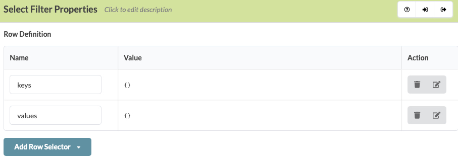
Select Add Dictionary Item , then select the Expression option from the drop-down menu to add the keys and values.
The following figure shows a keys definition (Remote_IP), with a single key. In this example, the value is
BFD.session_neighbor.Figure 1: Single-Key Example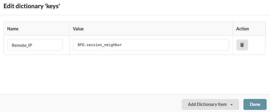
The following figure shows an example that defines four BFD values. In this example, the specified values are:
BFD.session_state,BFD.remote_state,BFD.session_type, andBGP.table_name.Figure 2: Four BFD Values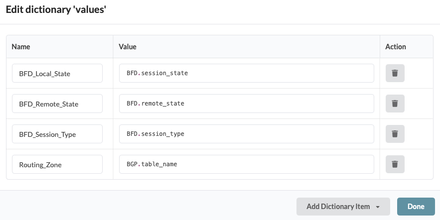
By defining values with a direct mapping to the accessor variables, the telemetry service produces output that exactly matches the originally ingested data.
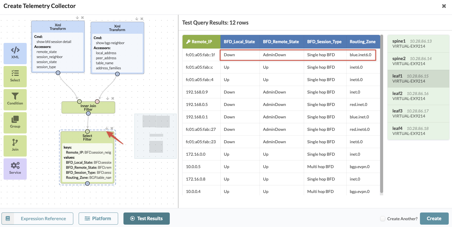
The Select Filter node enables advanced data transformation using Expression-based mapping. Use auto-completion and the Expression Reference page (lower left) for detailed examples and descriptions.
Link the Select Filter node to the Inner Join Filternode. On the Select Filter node, click the down arrow (Run up to this node).
Edit the values for each field.
Begin by identifying possible values for each value field and creating a schema to convert strings into numerical values This allows IBA to process data as a Discrete State and reverse the conversion.
We assigned numerical values to each state based on preference. You can assign values differently but must ensure symmetrical mapping in IBA. Consistent mapping is more important than specific values, as explained later. We'll create an expression to sequentially convert string values into numerical values for each state.
Note: Ensure the expression is written as one continuous line. This guide splits it into multiple lines for readability.The following figure illustrates BFD Session States (local) with four values: Up, Down, Init, and Failing.
Figure 3: BFD Local Session States with Four Values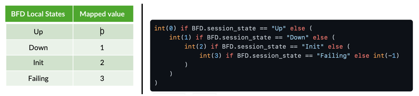
int(0) if BFD.session_state == "Up" else (
    int(1) if BFD.session_state == "Down" else (
        int(2) if BFD.session_state == "Init" else (
            int(3) if BFD.session_state == "Failing" else int(-1)
        )
     )
)
The following figure illustrates BFD Remote States with three possible values. Up, Down, and AdminDown.
Figure 4: BFD Remote States with Three Values
int(0) if BFD.session_state == "Up" else (
    int(1) if BFD.session_state == "Down" else (
        int(2) if BFD.remote_state == "AdminDown" else int(-1)
    )
)
The following figure illustrates BFD Session Types with two possible values: Single-Hop BFD and MultiHop BFD session types.
Figure 5: BFD Session Types with Two Values
int(1) if BFD.session_type == "Single hop BFD" else (
    int(2) if BFD.session_type == "Multi hop BFD" else int(-1)
)
Specify the mapping for the Routing Zone.
The data transformation in the Routing_Zone, which uses the BGP.table_name, will differ. In our example, we created a mapping between the BGP table names and descriptive strings.
The following figure shows five BGP tables:
inet.0,inet6.0,bgp.evpn.0,red.inet.0, andblue.inet.0. By mapping these table names to meaningful identifiers, we can easily determine whether a BFD session belongs to the default BGP table, an overlay BGP session, or a specific routing instance.Figure 6: Routing Zone Mapping
str('default') if 'inet' in BGP.table_name.split('.')[0] else (
    str('Overlay') if 'bgp' in BGP.table_name.split ('.')[0] else (
         BGP.table_name.split('.')[0]
    )
)
The following image shows the expected values dictionary configuration for expression-based mapping.
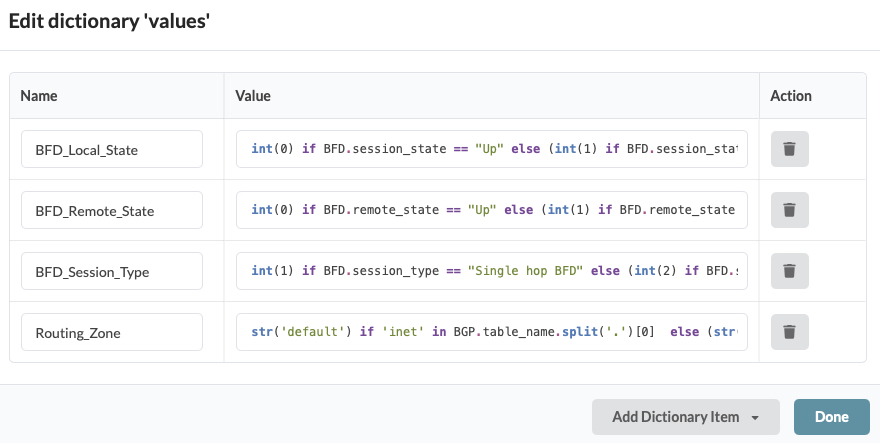
Test the results of the Select Filter node.
Note: The Test Query Results table has color-coded columns. Keys are shown in the green column, while values are shown in the blue column.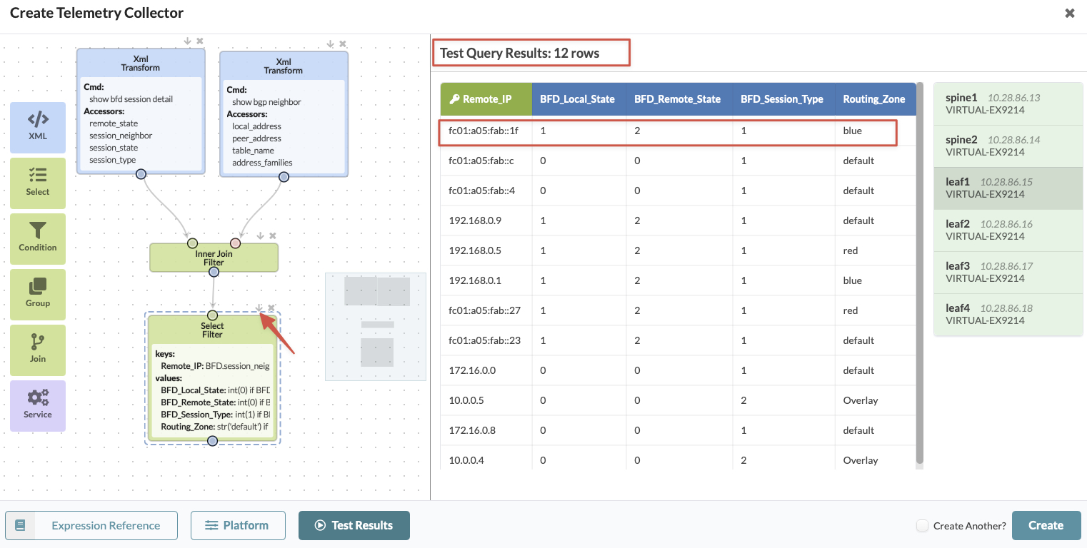
Publish the Results Using the Service Sink Node
To publish the results using the Service Sink node:
-
Select the Service Sink node icon on the
Create Telemetry page.
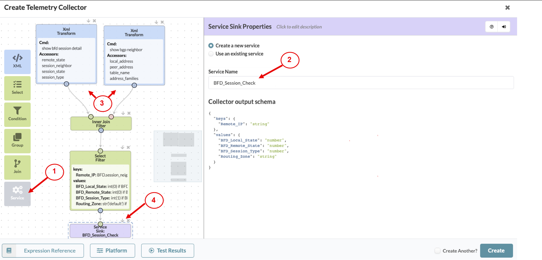
-
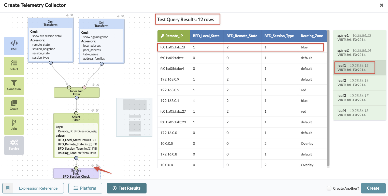
Verify the Service Sink node Test
Results. Click the down arrow (Run up to this node).
Select any device from the list to view the results, such as leaf1.
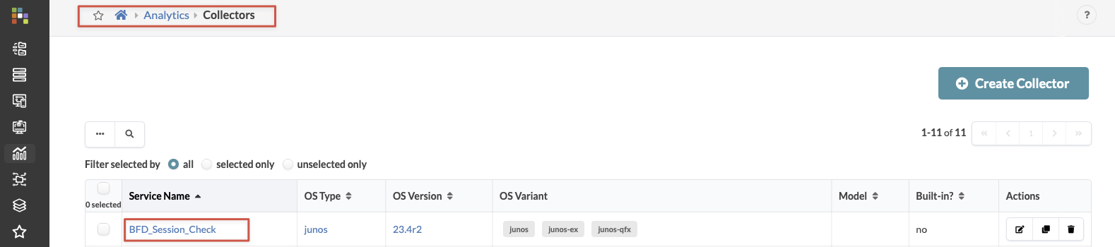
 The collector you just created appears on the Collectors page.
 The Service Registry displays the corresponding service. From the registry, you can view the service schema, including the keys and values.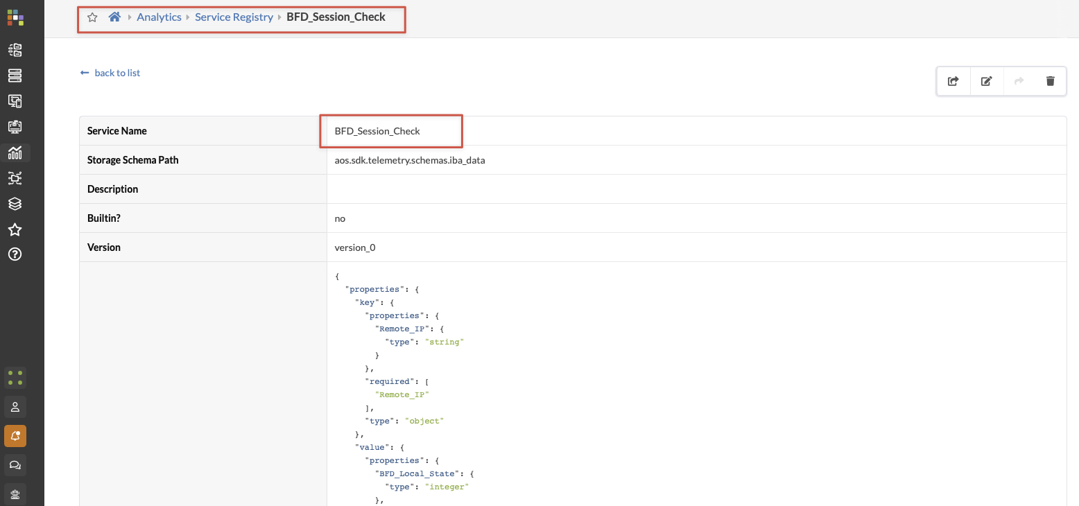
Next, continue to Create an IBA Probe and Processor.