Solution Architecture
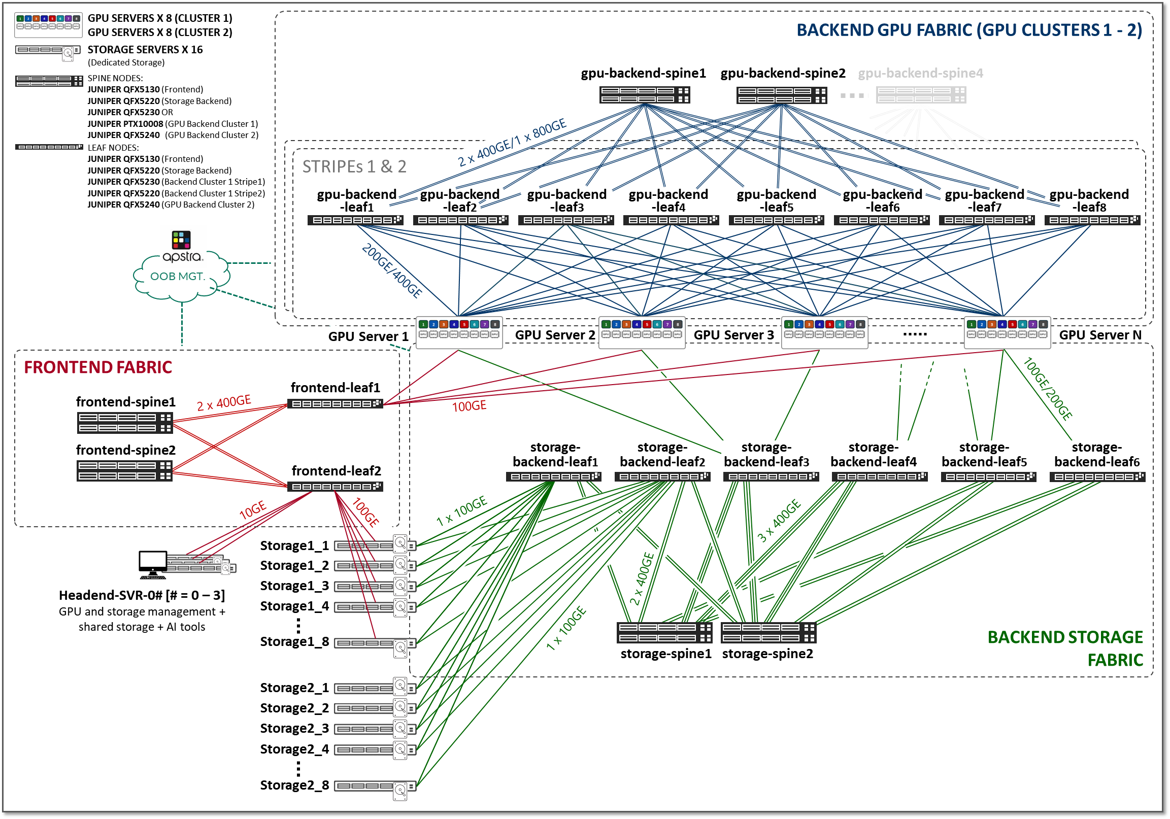
The three fabrics described in the previous section (Frontend, GPU Backend, and Storage Backend), are interconnected together in the overall AI JVD solution architecture shown in Figure 2.
Figure 2: AI JVD Solution Architecture
Frontend Fabric
The Frontend Fabric provides the infrastructure for users to interact with the AI systems to orchestrate training and inference tasks workflows using tools such as SLURM, Kubernetes, and other AI workflow managers that handle job scheduling, resource allocation, and lifecycle management.
These interactions do not generate heavy data flows and do not impose strict requirements on latency or packet loss. As a result, control-plane traffic does not place rigorous performance demands on the fabric.
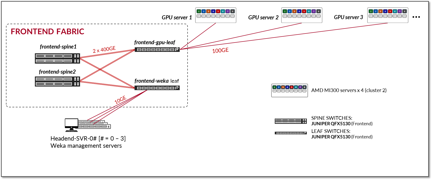
The Frontend Fabric design consists of a 3-stage L3 IP fabric without high availability (HA), as shown in Figure 3. This architecture provides a simple and effective solution for the connectivity required in the Frontend. However, any fabric architecture including EVPN/VXLAN, could be used. If an HA-capable Frontend Fabric is required, we recommend following the 3-Stage with Juniper Apstra JVD.
Figure 3: Frontend Fabric Architecture
The number of leaf nodes is dependent on the number of servers and storage devices in the AI cluster, as well as any other device used for AI job scheduling, resource allocation, and lifecycle management.
The number of spine nodes is dependent on the subscription factor desired for the design. A 1:1 subscription factor is not required. Moderate oversubscription is acceptable for control-plane traffic, provided the design maintains resiliency and avoids congestion that would impact control-plane stability.
The fabric is an L3 IP fabric using EBGP for route advertisement with IP addressing and EBGP configuration details described in the networking section on this document. No special load balancing mechanism is required. ECMP across redundant L3 paths is typically sufficient.
Given that the control-plane traffic is typically not bandwidth-heavy compared to storage or GPU fabrics, strict QoS mechanisms are optional and only recommended if sharing links with bursty non-control traffic.
The devices and connectivity in the Frontend fabric validated in this JVD are summarized in the following tables:
Table 1: Validated management devices and GPU servers connected to the Frontend fabric
| AMD GPU Servers | Headend Servers |
|---|---|
|
Supermicro AS-8125GS-TNMR2 AMD Instinct MI300X 192 GB OAM GPUs |
Supermicro SYS-6019U-TR4 |
Table 2: Validated Frontend Fabric leaf and spine nodes
| Frontend Leaf Nodes switch model | Frontend Fabric Spine Nodes switch model |
|---|---|
| QFX5130-32CD | QFX5130-32CD |
| QFX5220-32CD | QFX5220-32CD |
Table 3: Validated connections between headend servers and leaf nodes in the Frontend Fabric
| Links per GPU server to leaf connection | Server Type |
|---|---|
| 1 x 10GE | Supermicro SYS-6019U-TR4 |
Table 4: Validated connections between GPU servers and leaf nodes in the Frontend Fabric
| Links per GPU server to leaf connection | Server Type |
|---|---|
| 1 x 100GE | AMD Instinct MI300X |
Table 5: Validated connections between leaf and spine nodes in the Frontend Fabric
| Links per leaf and spine connection | Leaf node model | spine node model |
|---|---|---|
| 2 x 400GE | QFX5130-32CD | QFX5130-32CD |
Testing for this JVD was performed using 4 AMD Instinct MI300X GPU servers connected to two leaf nodes, which in turn were connected to two spine nodes, as shown:
Figure 4: Frontend JVD Testing Topology
- GPU servers are connected to the Leaf nodes using 100G interfaces (ConnectX-7 NICs).
- Vast devices are connected to the Leaf nodes using 100G interfaces
Table 6: Aggregate Frontend GPU Servers <=> Frontend Leaf Nodes Link Counts and bandwidth tested
| GPU Servers <=> Frontend Leaf Nodes | Bandwidth |
|---|---|
|
Number of 100GE links GPU servers ó frontend leaf nodes = 4 (1 per server) |
4 x 100GE = 400 Gbps |
|
Number of 100GE links between Storage device ó frontend leaf nodes = 8 (1 per storage device) |
8 x 100GE = 800 Gbps |
| Total bandwidth = | 1.0 Tbps |
Table 7: Aggregate Frontend Leaf Nodes <=> Frontend Spine Nodes Link Counts and bandwidth tested
| Frontend Leaf Nodes <=> Frontend Spine Nodes | Bandwidth | |
|---|---|---|
|
Number of 400GE links between frontend leaf nodes and spine nodes = 8 (2 leaf nodes x 2 spines nodes x 2 links per leaf to spine connection) |
8 x 400GE = 3.2 Tbps | |
| Total bandwidth = | 3.2 Tbps | |
| No over subscription | ||
GPU Backend Fabric
The GPU Backend fabric provides the infrastructure for GPUs to communicate with each other within a cluster, using RDMA over Converged Ethernet (RoCEv2). RoCEv2 enhances data center efficiency, reduces complexity, and optimizes data delivery across high-speed Ethernet networks.
Unlike the Frontend Fabric, the GPU Backend Fabric carries data-plane traffic that is both bandwidth-intensive and latency-sensitive. Packet loss, excessive latency, or jitter can significantly impact job completion times and therefore must be avoided.
As a result, one of the primary design objectives of the GPU Backend Fabric is to provide a near-lossless Ethernet fabric, while also delivering maximum throughput, minimal latency, and minimal network interference for GPU-to-GPU traffic. RoCEv2 operates most efficiently in environments where packet loss is minimized, directly contributing to optimal job completion times.
The GPU Backend Fabric in this JVD was designed to meet these requirements. The design follows a 3-stage IP Clos, Rail Optimized Stripe architecture , as shown in Figure 5. Details about the Rail Optimized Stripe architecture are described in a later section.
Figure 5: GPU Backend Fabric Architecture
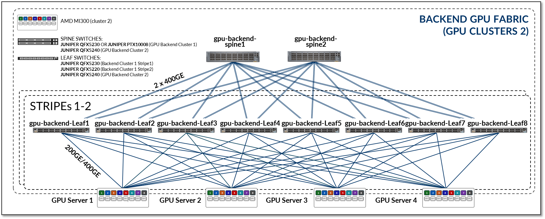
The fabric operates as an L3 IP fabric using EBGP for route advertisement with IP addressing and EBGP configuration details described in the networking section on this document.
In a rail optimized architecture, the number of leaf nodes is determined by the number of GPU per server, which is 8 for the AMD servers included in this JVD. The number of spine nodes as well as the speed and number of links between GPU servers and leaf nodes, and between leaf and spine nodes, determines the effective bandwidth and oversubscription characteristics of the GPU Backend Fabric.
In contrast to the Frontend Fabric, the GPU Backend Fabric typically targets a non-oversubscribed (1:1) design, or a very low oversubscription ratio. This ensures sufficient bandwidth for simultaneous collective operations and prevents congestion that could introduce packet loss or latency variation.
The fabric is an L3 IP fabric using EBGP for route advertisement with IP addressing and EBGP configuration details described in the networking section on this document. Traffic distribution within the GPU Backend Fabric relies on ECMP across multiple equal-cost L3 paths combined with advanced Load Balancing techniques such as Dynamic Load Balancing (DLB), Global Load Balancing, and Adaptive Load Balancing (ALB). These are described in the Load Balancing section of this document.
Because the GPU Backend Fabric carries RoCEv2 traffic sensitive to losses and latency, the design incorporates DCQCN (Data Center Quantized Congestion Notification), which leverages ECN (Explicit Congestion Notification) and may optionally use PFC (Priority Flow Control), to achieve lossless or near-lossless behavior for RDMA traffic. These mechanisms are described in detail in the Class of Service section of this document.
The devices and connectivity in the Frontend fabric validated in this JVD are summarized in the following tables:
Table 8: Validated management devices and GPU servers connected to the GPU Backend Fabric
| GPU Servers | Storage Devices | Headend Servers |
|---|---|---|
|
Supermicro AS-8125GS-TNMR2 AMD Instinct MI300X 192 GB OAM GPUs |
|
Supermicro SYS-6019U-TR4 |
Table 9: Validated GPU Backend Fabric Leaf Nodes
| GPU Backend Fabric Leaf Nodes switch model |
|---|
| QFX5220-32CD |
| QFX5230-64CD |
| QFX5240-64OD |
| QFX5241-64OD |
Table 10: Validated GPU Backend Fabric Spine Nodes
| GPU Backend Spine Fabric Nodes switch model |
|---|
| QFX5230-64CD |
| QFX5240-64OD |
| QFX5241-64OD |
| PTX10008 LC1201 |
| PTX10008 LC1301 |
Table 11: Validated connections between GPU servers and Leaf Nodes in the GPU Backend Fabric
| Links per GPU server to leaf connection | Server type |
|---|---|
| 1 x 400GE links per GPU server to leaf connection | AMD MI300 |
Table 12: Validated connections between leaf and spine nodes in the GPU Backend Fabric
| Links per leaf and spine connection | Leaf node model | Spine node model |
|---|---|---|
| 1 x 400GE | QFX5220-32CD | QFX5230-32CD |
| 1 x 400GE | QFX5230-32CD | QFX5230-32CD |
| 2 x 400GE | QFX5240-64OD | QFX5240-64OD |
| 1 x 800GE | QFX5240-64OD | QFX5240-64OD |
| 1 x 400GE | QFX5220-32CD | PTX10008 LC1201 |
| 1 x 400GE | QFX5230-32CD | PTX10008 LC1201 |
| 1 x 800GE | QFX5240-64OD | PTX10008 LC1301 |
| 2 x 800GE | QFX5240-64OD | PTX10008 LC1301 |
Testing for this JVD was performed using 4 MI300 GPU servers connected to two stripes as shown:
Figure 6: GPU Backend JVD Testing Topology
- Each AMD MI300X GPU server is connected to the Leaf nodes using 400G interfaces (Thor2 and Pollara NICs).
validated_optics_summary.html#Toc222928841__DAC_5m were tested with Broadcom Thor2 cards and connected as shown in the diagram below.
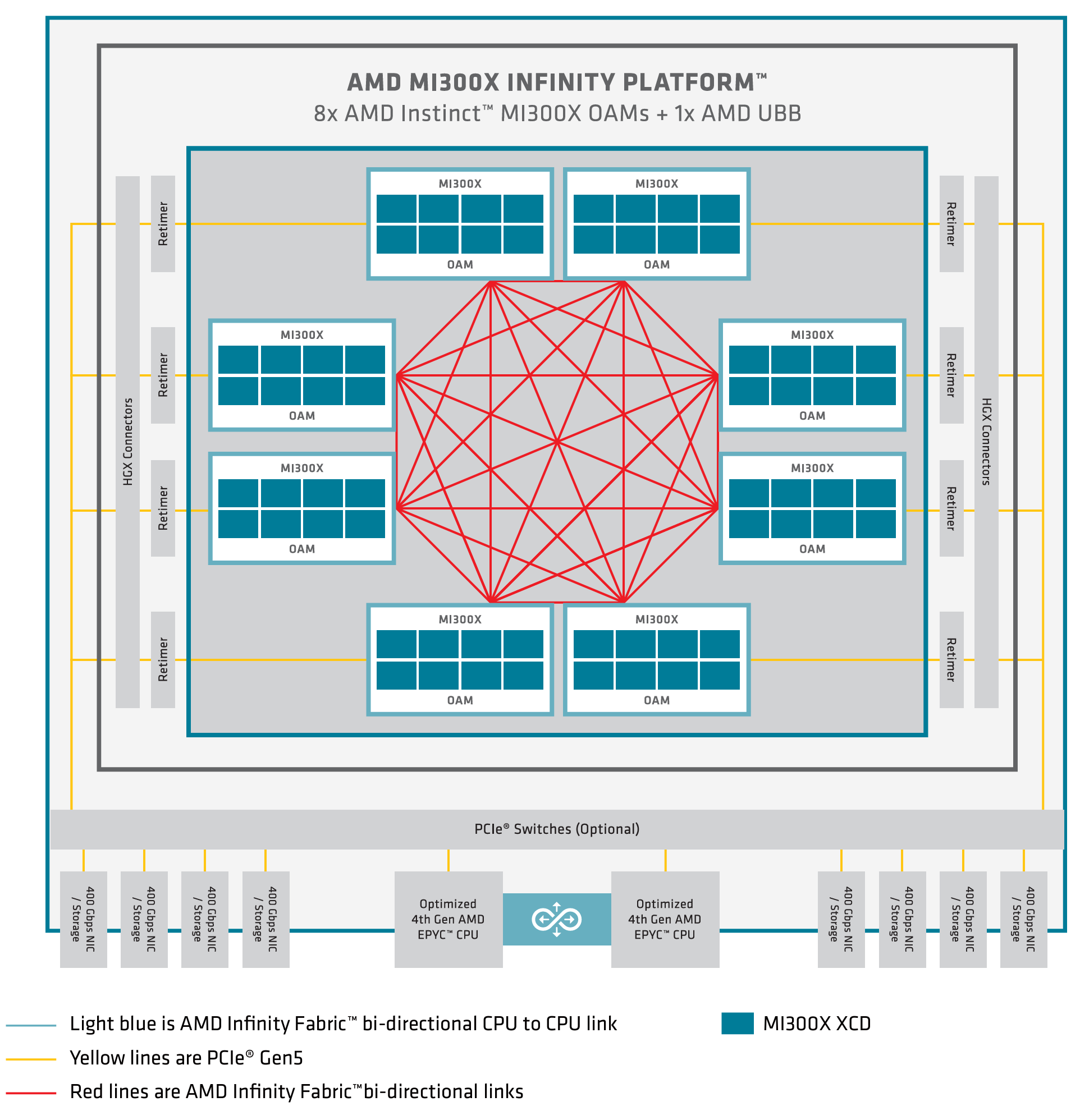
Table 13: Per stripe Server to Leaf Bandwidth
| Stripe |
Number of servers per Stripe |
Number of servers <=> leaf links per server (number of leaf nodes & number of GPUs per server) |
Server <=> Leaf Link Bandwidth [Gbps] |
Total Servers <=> Leaf Links Bandwidth per stripe [Tbps] |
|---|---|---|---|---|
| 1 | 2 MI300 | 8 | 400 Gbps | 2 x 8 x 400 Gbps = 6.4 Tbps |
| 2 | 2 MI300 | 8 | 400 Gbps | 2 x 8 x 400 Gbps = 6.4 Tbps |
| Total Server <=> Leaf Bandwidth | 12.8 Tbps | |||
Table 14: Per stripe Leaf to Spine Bandwidth w/ QFX5240 as leaf and spines
| Stripe |
Number of leaf nodes |
Number of spine nodes |
Number of 400 Gbps leaf <=> spine links per leaf node |
Server <=> Leaf Link Bandwidth [Gbps] |
Bandwidth Leaf <=> Spine Per Stripe [Tbps] |
|---|---|---|---|---|---|
| 1 | 8 | 4 | 2 | 400 | 8 x 2 x 2 x 400 Gbps = 12.8Tbps |
| 2 | 8 | 4 | 2 | 400 | 8 x 2 x 2 x 400 Gbps = 12.8Tbps |
| Total Server <=> Leaf Bandwidth | 25.6 Tbps | ||||
GPU Backend Fabric Subscription Factor
The subscription factor is simply calculated by comparing the numbers from the two tables above:
In the JVD test environment, the bandwidth between the servers and the leaf nodes is 6.4 Tbps per stripe, while the bandwidth available between the leaf and spine nodes is 12.8 Tbps per stripe. This means that the fabric has enough capacity to process all traffic between the GPUs even when this traffic was 100% inter-stripe, while still having extra capacity to accommodate additional servers without becoming oversubscribed. The subscription factor in this case is 1:2.
Figure 7: 1:2 subscription factor (over-provisioned)
To run oversubscription testing, some of the interfaces between the leaf and spines were disabled, reducing the available bandwidth, as shown in the example in Figure 8:
Figure 8: 1:1 Subscription Factor
Additionally, an Ixia traffic generator emulating RoCEv2 devices was also connected to the fabric, as shown in the example in Figure 9.
Figure 9: 1:1 Subscription Factor
This adds an additional 800G of traffic to leafs 2 and 4 on both stripes 1, and 2.
GPU to GPU Communication Optimization
Optimization in rail-optimized topologies refers to how GPU communication is managed to minimize congestion and latency while maximizing throughput. A key part of this optimization strategy is keeping traffic local whenever possible. By ensuring that GPU communication remains within the same rail or stripe, or even within the server, the need to traverse spines or external links is reduced, which lowers latency, minimizes congestion, and enhances overall efficiency.
While localizing traffic is prioritized, inter-stripe communication will be necessary in larger GPU clusters. Inter-stripe communication is optimized by means of proper routing and balancing techniques over the available links to avoid bottlenecks and packet loss.
The essence of optimization lies in leveraging the topology to direct traffic along the shortest and least-congested paths, ensuring consistent performance even as the network scales. Traffic between GPUs on the same servers can be forwarded locally across the internal Server fabric (vendor dependent), while traffic between GPUs on different servers happens across the external GPU backend infrastructure. Communication between GPUs on different servers can be intra-rail, or inter-rail/inter-stripe.
Intra-rail traffic is switched (processed at Layer 2) on the local leaf node. Following this design, data between GPUs on different servers (but in the same stripe) is always moved on the same rail and across one single switch. This guarantees GPUs are 1 hop away from each other and will create separate independent high-bandwidth channels, which minimize contention and maximize performance. On the other hand, inter-rail/inter-stripe traffic is routed across the IRB interfaces on the leaf nodes and the spine nodes connecting the leaf nodes (processed at Layer 3).
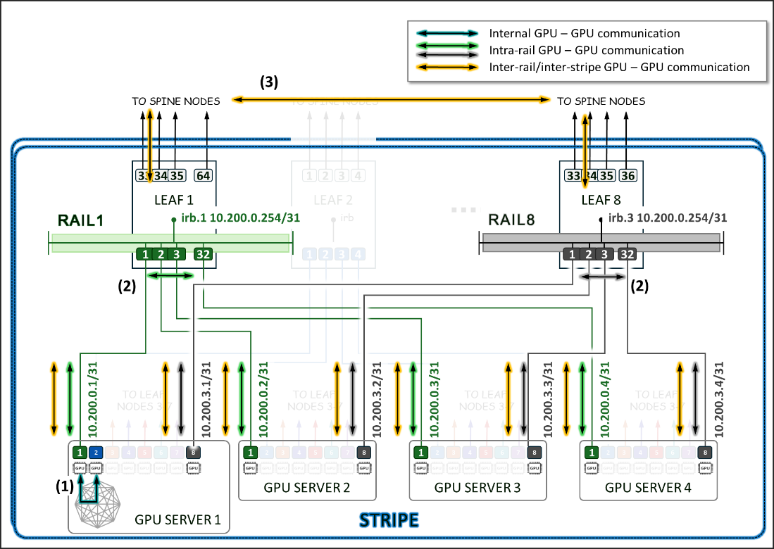
Consider the example depicted in Figure 10
- Communication between GPU 1 and GPU 2 in server 1 happens across the server’s internal fabric (1),
- Communication between GPUs 1 in servers 1- 4, and between GPUs 8 in servers 1- 4 happens across Leaf 1 and Leaf 8 respectively (2), and
- Communication between GPU 1 and GPU 8 (in servers 1- 4) happens across leaf1, the spine nodes, and leaf8 (3)
Figure 10: Inter-rail vs. Intra-rail GPU-GPU communication
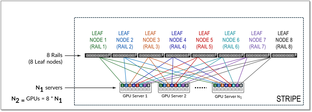
Figure 10 represents a topology with one stripe and 8 rails connecting GPUs 1-8 across leaf switches 1-8, respectively.
Communication between GPU 7 and GPU 8 in Server 1 happens across the internal fabric, while communication between GPU 1 in Server 1 and GPU 1 in Server N1 happens across Leaf switch 1 (within the same rail).
Notice that if any communication between GPUs in different stripes and different servers is required (e.g. GPU 4 in server 1 communicating with GPU 5 in Server N1), data is first moved to a GPU interface in the same rail as the destination GPU, thus sending data to the destination GPU without crossing rails.
Following this design, data between GPUs on different servers (but in the same stripe) is always moved on the same rail and across one single switch, which guarantees GPUs are 1 hop away from each other and creates separate independent high-bandwidth channels, which minimize contention and maximize performance.
On AMD GPU servers, GPUs are interconnected via the AMD Infinity fabric, which provides 7x128GB/s GPU-to-GPU high-bandwidth, low-latency, and bidirectional GPU-to-GPU communication within a single server, as shown in Figure 11.
Figure 11. AMD MI300X architecture.
For more details refer to AMD Instinct™ MI300 Series microarchitecture — ROCm Documentation
AMD MI300X GPUs leverage Infinity Fabric, providing high-bandwidth, low-latency communication between GPUs, CPUs, and other components. This interconnect can dynamically manage traffic prioritization across links, providing an optimized path for communication within the node.
By default, AMD MI300X devices implement local optimization to minimize latency for GPU-to-GPU traffic. Communication between GPUs on the same servers is forwarded across the Infinity Fabric and remains intra-node and does not traverse the external Ethernet fabric. Traffic between GPUs of the same rank across multiple servers remains intra-stripe.
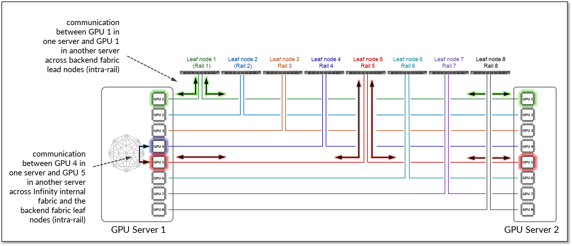
Figure 12 shows an example where GPU1 in Server 1 communicates with GPU1 in Server 2. The traffic is forwarded by Leaf Node 1 and remains within Rail 1.
Additionally, if GPU4 in Server 1 wants to communicate with GPU5 in Server 2, and GPU5 in Server 1 is available as a local hop in AMD’s Infinity Fabric, the traffic naturally prefers this path to optimize performance and keep GPU-to-GPU communication intra-rail.
Figure 12: GPU to GPU inter-rail communication between two servers with local optimization.
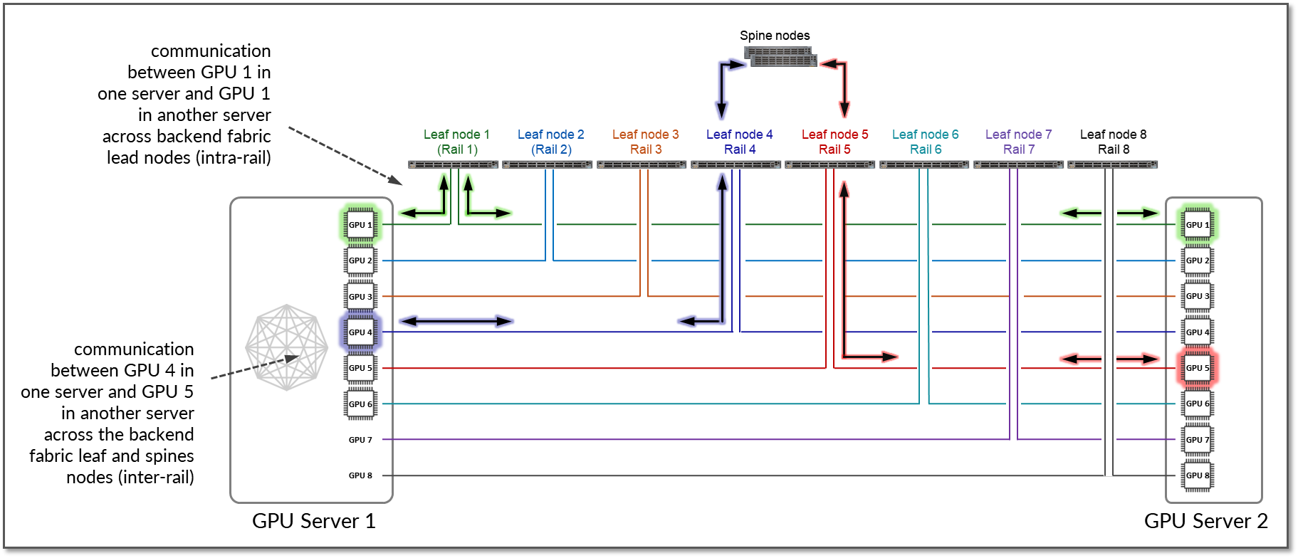
If local optimization is not feasible because of workload constraints, for example, the traffic must bypass local hops (internal fabric) and use RDMA (off-node NIC-based communication). In such a case, GPU4 in Server 1 communicates with GPU5 in Server 2 by sending data directly over the NIC using RDMA, which is then forwarded across the fabric, as shown in Figure 13.
Figure 13: GPU to GPU inter-rail communication between two servers without local optimization.
The example shows that communication between GPU 4 in Server 1 and GPU 5 in Server N1 goes across Leaf switch 1, the Spine nodes, and Leaf switch 5 (between two different rails).
Backend GPU Rail Optimized Architecture
As previously described, a Rail Optimized Stripe Architecture provides efficient data transfer between GPUs, especially during computationally intensive tasks such as AI Large Language Models (LLM) training workloads, where seamless data transfer is necessary to complete the tasks within a reasonable time. A Rail Optimized topology aims to maximize performance by providing minimal bandwidth contention, minimal latency, and minimal network interference, ensuring that data can be transmitted efficiently and reliably across the network.
In a Rail Optimized Architecture, there are two important concepts: rail and stripe.
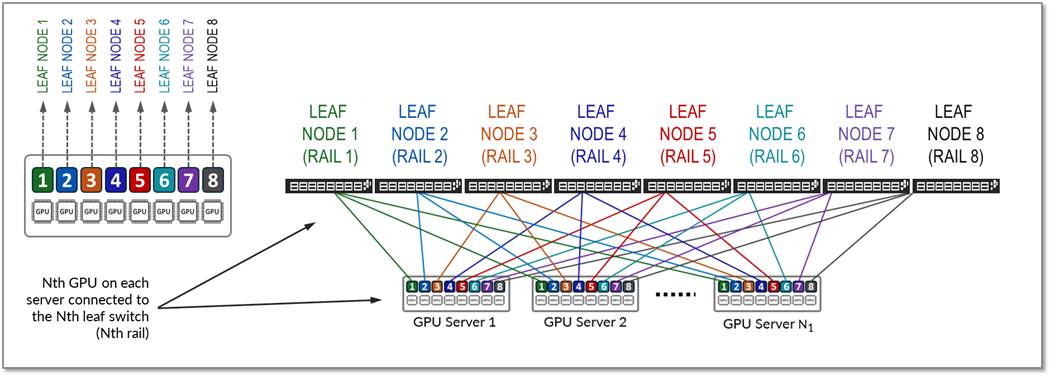
The GPUs on a server are numbered 1-8, where the number represents the GPU’s position in the server, as shown in Figure 14. This number is sometimes called rank or more specifically "local rank" in relationship to the GPUs in the server where the GPU sits, or "global rank" in relationship to all the GPUs (in multiple servers) assigned to a single job.
A rail connects GPUs of the same order across one of the leaf nodes in the fabric; that is, rail Nth connects all GPU in position Nth on all the servers, to leaf node Nth, as shown in Figure 14.
Figure 14: Rails in a Rail Optimized Architecture

A stripe refers to a design module or building block, comprised of multiple rails, and includes Leaf nodes and GPU servers, as shown in Figure 15. This building block can be replicated to scale up the AI cluster.
Figure 15: Stripes in a Rail Optimized Architecture
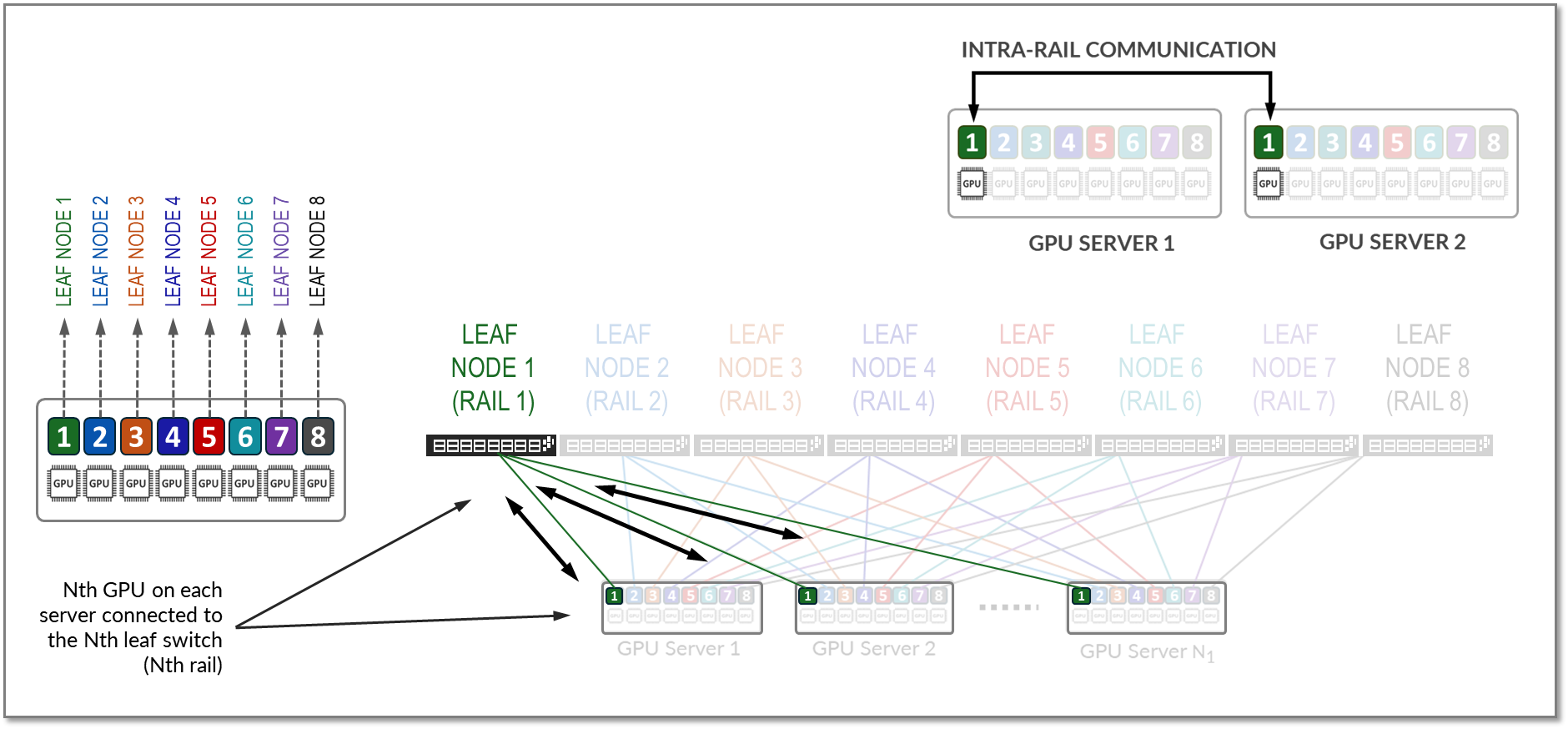
All traffic between GPUs of the same rank (intra-rail traffic) is forwarded at the leaf node level as shown in Figure 16.
Figure 16: Intra-rail traffic example.
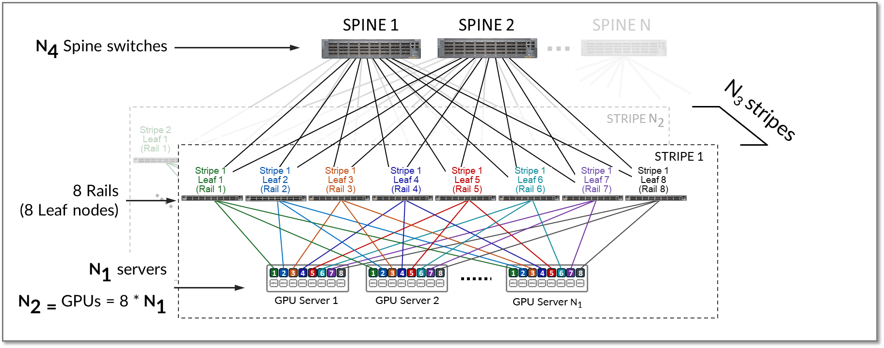
A stripe can be replicated to scale up the number of servers (N1) and GPUs (N2) in an AI cluster. Multiple stripes (N3) are then connected across Spine switches as shown in Figure 17.
Figure 17: Multiple stripes connected via Spine nodes
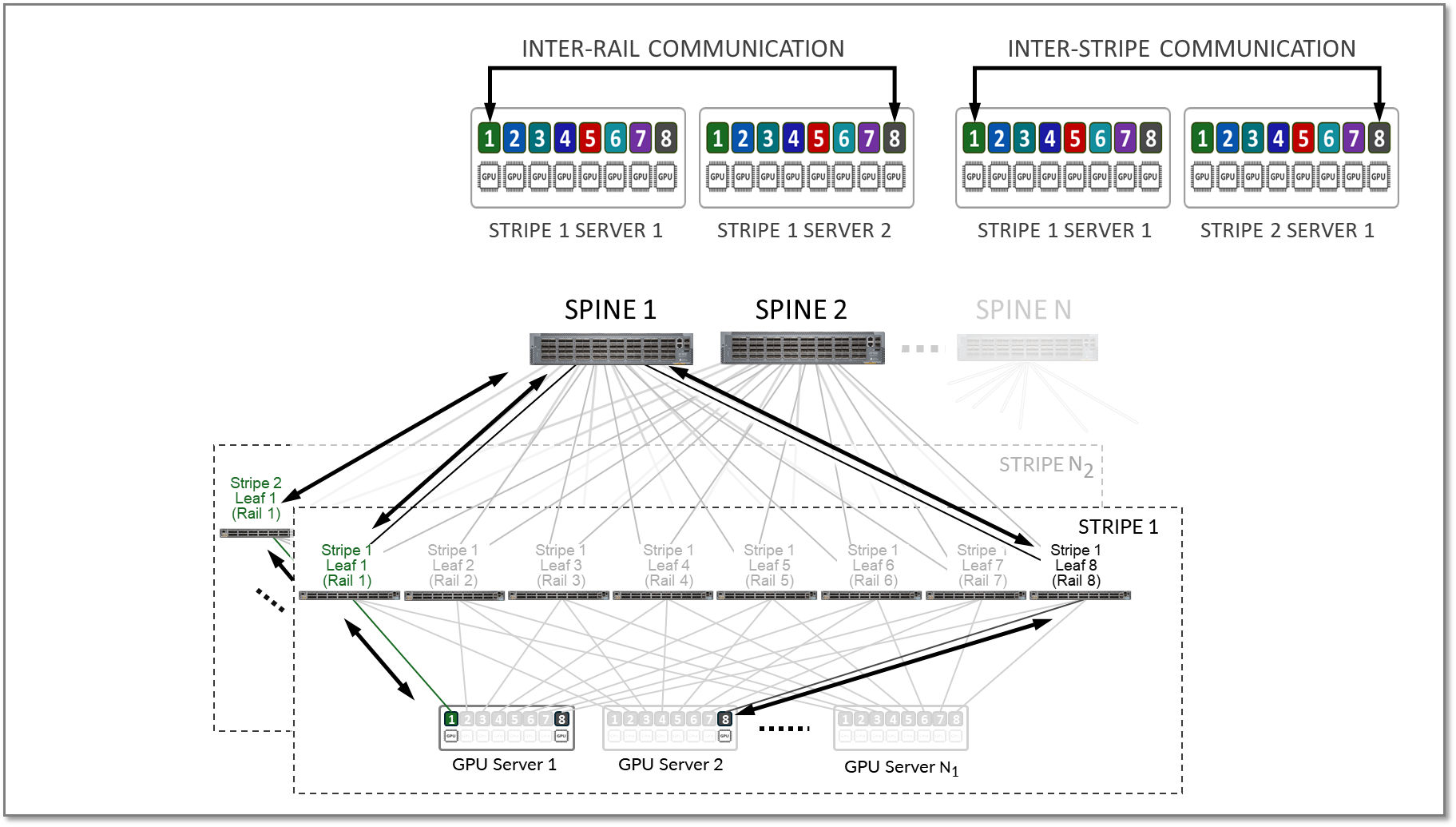
Both Inter-rail and inter-stripe traffic will be forwarded across the spines nodes as shown in figure 18.
Figure 18. Inter-rail, and Inter-stripe GPU to GPU traffic example.
Calculating the number of leaf and spine nodes, Servers, and GPUs in a rail optimized architecture
The number of leaf nodes in a single stripe in a rail optimized architecture is defined by the number of GPUs per server (number of rails). Each AMD MI300X GPU server includes 8 AMD Instinct MI300X GPUs. Therefore, a single stripe includes 8 leaf nodes (8 rails).
Number of leaf nodes = number of GPUs x server = 8
The maximum number of servers supported in a single stripe (N1) is defined by the number of available ports on the Leaf node which depends on the switches model.
The total bandwidth between the GPU servers and leaf nodes must match the total bandwidth between leaf and spine nodes to maintain a 1:1 subscription ratio.
Assuming all the interfaces on the leaf node operate at the same speed, half of the interfaces will be used to connect to the GPU servers, and the other half to connect to the spines. Thus, the maximum number of servers in a stripe is calculated as half the number of available ports on each leaf node.
Figure 19. Number of uplinks and downlinks for 1:1 subscription factor
In the diagram, X represents the number of downlinks (links between leaf nodes and the GPU servers), while Y represents the number of uplinks (links between the leaf nodes and the spine nodes). To allow for a 1:1 subscription factor, X must be equal to Y.
The number of available ports on each leaf node is equal to X + Y or 2 * X.
Because all servers in a stripe have one port connected to every leaf in the stripe, the maximum number of servers in the stripe (N1) is equal to X.
N1 (maximum number of servers per stripe) = number of available ports ÷ 2
The maximum number of GPUs in the stripe is calculated by simply multiplying the number of GPUs per server.
N2 (maximum number of GPUs) = N1 (maximum number of servers per stripe) * 8
The total number of available ports is dependent on the switch model used for the leaf node. Table 15 shows some examples.
Table 15: Maximum number of GPUs supported per stripe
|
Leaf Node QFX switch Model |
number of available 400 GE ports per switch |
Maximum number of servers supported per stripe for 1:1 Subscription (N1) |
GPUs per server |
Maximum number of GPUs supported per stripe (N2) |
|---|---|---|---|---|
| QFX5220-32CD | 32 | 32 ÷ 2 = 16 | 8 | 16 servers x 8 GPUs/server = 128 GPUs |
| QFX5230-64CD | 64 | 64 ÷ 2 = 32 | 8 | 32 servers x 8 GPUs/server = 256 GPUs |
|
QFX5240-64OD QFX5241-64OD |
128 | 128 ÷ 2 = 64 | 8 | 64 servers x 8 GPUs/server = 512 GPUs |
- QFX5220-32CD switches provide 32 x 400 GE ports => 16 will be used to connect to the servers and 16 will be used to connect to the spine nodes.
- QFX5230-64CD switches provide up to 64 x 400 GE ports => 32 will be used to connect to the servers and 32 will be used to connect to the spine nodes.
- QFX5240-64OD switches provide up to 128 x 400 GE ports => 64 will be used to connect to the servers and 64 will be used to connect to the spine nodes.
To achieve larger scales, multiple stripes (N3) can be connected using a set of Spine nodes (N4), as shown in Figure 20.
Figure 20. Multiple Stripes connected across Spine nodes
The number of stripes required (N3 ) is calculated based on the required number of GPUs, and the maximum number of GPUs per stripe (N2).
For example, assume that the required number of GPUs (GPUs) is 16,000, and the fabric is using QFX5240-64OD as leaf nodes.
The number of available 400G ports is 128 which means that:
- maximum number of servers per stripe (N1) = 64
- maximum number of GPUs per stripe (N2) = 512
The number of stripes (N3) required is calculated by dividing the number of GPUs required, and the number of GPUs per stripe as shown:
N 3 (number of stripes required) = GPUs ÷ N 2 (maximum number of GPUs per stripe) = 16000 ÷ 512 = 32 stripes (rounded up)
- With 32 stripes and 64 servers per stripe, the cluster can provide 16,384 GPUs.
Knowing the number of stripes required (N 3) and the number of uplinks ports per leaf node (Y) you can calculate how many spine nodes are required.
Remember X = Y = N1
First the total number of leaf nodes can be calculated by multiplying the number of stripes required by 8 (number of leaf nodes per stripe).
Total number of leaf nodes = N3 x 8 = 32 x 8 = 256
Then the total number of uplinks can be obtained multiplying the number of uplinks per leaf node (N1), and the total number of leaf nodes.
Total number of uplinks = N1 x 256 = 64 x 256 = 16384
The number of spines required (N4 ) can then be determined by dividing the total number of uplinks by the number of available ports on each spine node, which as for the leaf nodes, depends on the switch model used for the spine role.
Number of spines required (N4 ) = 16384 / number of available ports on each spine node
For example, if the spine nodes are QFX5240/41, the number of available ports on each spine node is 128.
Table 16: Number of spines nodes for two stripes.
|
Spine Node QFX switch Model |
Maximum number of 400 GE interfaces per switch | Number of spines required (N4) with 64 stripes |
|---|---|---|
| QFX5240-64OD | 128 | 16384 ÷ 128 = 128 |
| PTX10008 LC1201 | 288 | 16384 ÷ 288 ~ 57 |
| PTX10008 LC1301 | 576 | 16384 ÷ 576 ~ 29 |
Storage Backend Fabric
The Storage Backend fabric provides the connectivity infrastructure for storage devices to be accessible from the GPU servers.
The performance of the storage infrastructure significantly impacts the efficiency of AI workflows. A storage system that provides quick access to data can significantly reduce the amount of time for training AI models. Similarly, a storage system that supports efficient data querying and indexing can minimize the completion time of preprocessing and feature extraction in an AI workflow.
In small clusters, it may be sufficient to use the local storage on each GPU server, or to aggregate this storage together using open-source or commercial software. In larger clusters with heavier workloads, an external dedicated storage system is required to provide dataset staging for ingest, and for cluster checkpointing during training.
Two leading platforms, WEKA and Vast Storage, provide cutting-edge solutions for shared storage in GPU environments. While we have tested both solutions in our lab, this JVD focuses on the Vast Storage Solution. Thus, the rest of this, as well as other sections in this document, will cover details about Vast Storage devices and connectivity to the Storage Backend Fabric.
Details about the WEKA storage are included in the AI Data Center Network with Juniper Apstra, NVIDIA GPUs, and WEKA Storage—Juniper Validated Design (JVD).
The Storage Backend Fabric design in the JVD also follows a 3-stage IP clos architecture as shown in Figure 21. There is no concept of rail-optimization in a storage cluster. Each GPU server has single connections to the leaf nodes, instead of one connection per GPU.
Figure 21: Storage Backend Fabric Architecture
The number of leaf nodes depends on the GPU number of servers and storage devices in the AI cluster.
The number of spine nodes is dependent on the subscription factor desired for the design. Like the GPU Backend Fabric, the Storage Fabric requires a non-oversubscribed design (1:1 subscription factor) to ensure sufficient bandwidth for the high-volume traffic, and to prevent congestion, packet loss, and excessive latency.
Storage traffic can use different transport mechanisms, including NFS, POSIX, and RoCEv2. For RoCEv2, the same Load Balancing and Class of Service mechanisms described for the GPU Backend fabric must be implemented. These are described in the Load Balancing and Class of Service sections of this document.
The devices and connectivity in the Storage Fabric validated in this JVD are summarized in the following tables:
Table 17: Validated Storage Fabric leaf and spine nodes
| Storage Fabric Leaf Nodes switch model | Storage Fabric Spine Nodes switch model |
|---|---|
| QFX5130-32CD | QFX5130-32CD |
| QFX5220-32CD | QFX5220-32CD |
| QFX5230-32CD | QFX5230-32CD |
| QFX5240-64OD | QFX5240-64OD |
Table 18: Validated connections between GPU servers, and storage devices, and leaf nodes in the Storage Fabric
| Links per GPU server to leaf connection | Server Type |
|---|---|
| 1 x 100GE | VAST c-nodes |
| 1 x 200GE | AMD MI300 GPU servers |
Table 19: Validated connections between leaf and spine nodes in the Storage Fabric
| Links per leaf and spine connection | Leaf node model | spine node model |
|---|---|---|
| 2 x 400GE, 3 x 400GE | QFX5130-32CD | QFX5130-32CD |
| 2 x 400GE, 3 x 400GE | QFX5130-32CD | QFX5130-32CD |
| 2 x 400GE, 3 x 400GE |
QFX5240-32CD QFX5241-32CD |
QFX5240-32CD QFX5241-32CD |
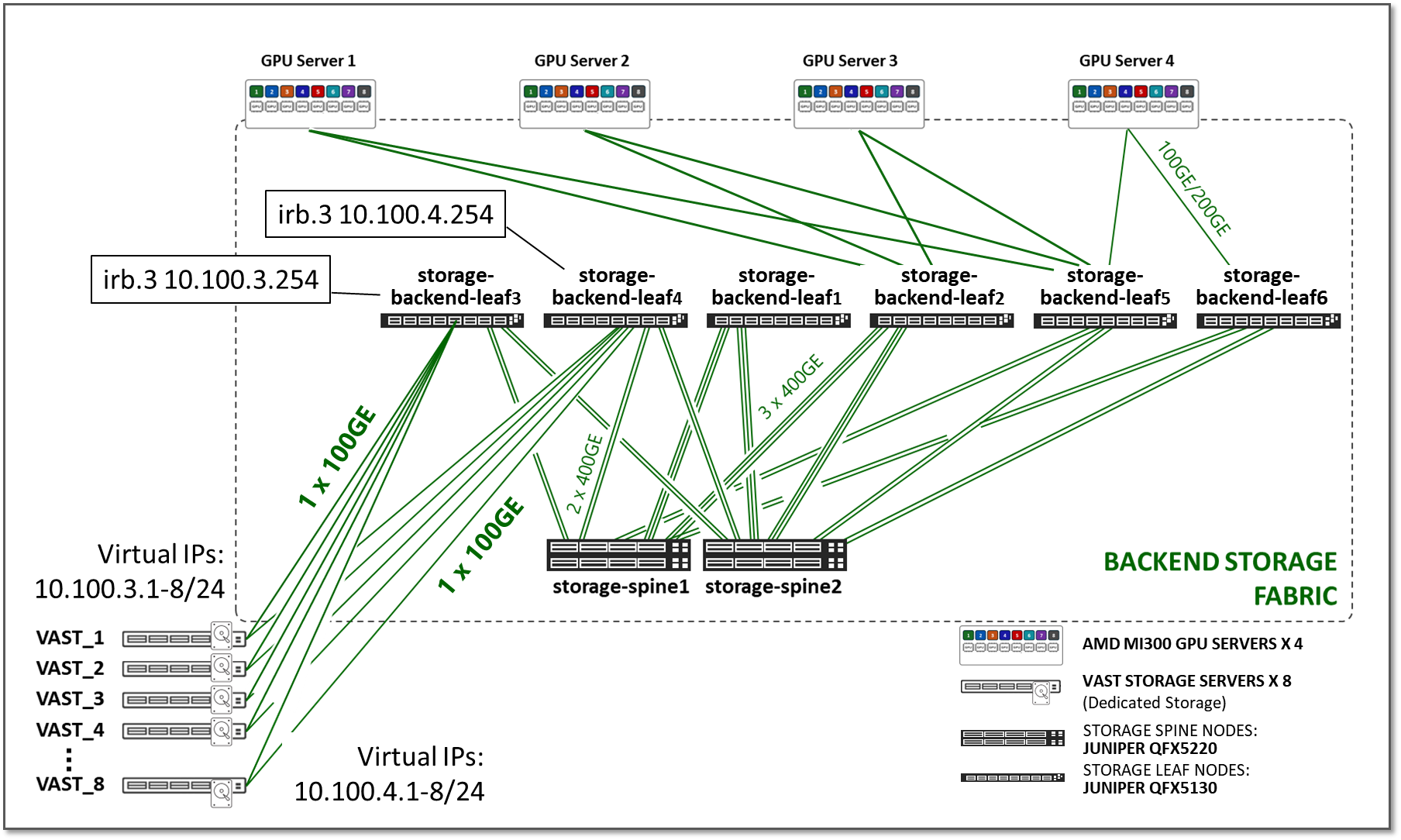
Testing for this JVD was performed using 4 AMD Instinct MI300X GPU servers and 8 VAST storage devices, connected to 4 leaf nodes, which in turn were connected to 2 spine nodes, as shown in Figure 22:
Figure 22: Storage Fabric JVD Testing Topology
Table 20: Aggregate Storage Link Counts and bandwidth tested
| GPU Servers <=> Storage Leaf Nodes | Storage Leaf Nodes <=> Frontend Spine Nodes |
|---|---|
|
Total number of 200GE links between GPU servers and storage leaf nodes = 4 (1 link per server) + Total number of 100GE links between Vast storage devices and storage leaf nodes (2 links per devices) = 16 |
Total number of 400GE links between frontend leaf nodes and spine nodes = 16 (2 links per leaf to spine connection) |
| Total bandwidth = 2.4 Tbps | Total bandwidth = 6.4 Tbps |
| No oversubscription. |
GPU Backend Fabric Scaling
The size of an AI cluster varies significantly depending on the specific requirements of the workload. The number of nodes in an AI cluster is influenced by factors such as the complexity of the machine learning models, the size of the datasets, the desired training speed, and the available budget. The number varies from a small cluster with less than 100 nodes to a data center-wide cluster comprised of 10000s of compute, storage, and networking nodes. A minimum of 4 spines must always be deployed for path diversity and reduction of PFC failure paths.
Table 21: Fabric Scaling- Devices and Positioning
| Fabric Scaling | ||
|---|---|---|
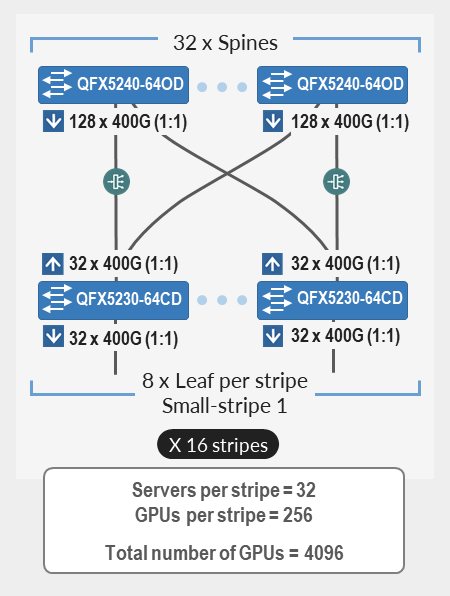
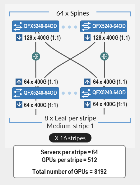
| Small | Medium | Large |
| up to 4096 GPU | up to 8192 GPU | 8192 and up to 73,728 GPU |
|
Support for up to 4096 GPUs with Juniper QFX5240-64CDs as spine nodes and QFX5230-64CD as leaf nodes (single or multi-stripe implementations). This 3-stage rail-based fabric consists of up to 32 Spines and 128 leaf nodes, maintaining a 1:1 subscription. The fabric provides physical connectivity for up to 16 stripes, with 32 servers (256 GPUs) per stripe, for a total of 4096 GPUs. |
Support for more than 4096 GPU and up to 8192 GPUs with Juniper QFX5240-64CDs as both Spine and Leaf nodes. This 3-stage rail-based fabric consists of up to 64 spines, and up to 128 leaf nodes, maintaining a 1:1 subscription. The fabric provides physical connectivity for up to 16 Stripes, with 64 servers (512 GPUs) per stripe, for a total of 8192 GPUs |
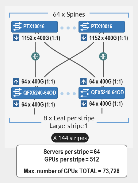
Support of more than 8192 GPU and up to. 73,728 GPUs with Juniper PTX10000 Chassis as Spine nodes and Juniper QFX5240-64CDs as leaf nodes. This 3-stage rail-based fabric consists of up to 64 spines, and up to 1152 leaf nodes, maintaining a 1:1 subscription. The fabric provides physical connectivity for up to 144 Stripes, with 64 servers (512 GPUs) per stripe, for a total of 73,728 GPUs. |
|
|
|
Validated Juniper Hardware and Software Solution Components
The Juniper products and software versions listed below pertain to the latest validated configuration for the AI DC use case. As part of an ongoing validation process, we routinely test different hardware models and software versions and update the design recommendations accordingly.
The version of Juniper Apstra in the setup is 6.1.
The following table summarizes the validated Juniper devices for this JVD and includes devices tested for the AI Data Center Network with Juniper Apstra, NVIDIA GPUs, and WEKA Storage—Juniper Validated Design (JVD).
Table 22: Validated Devices and Positioning
| DEVICE | FRONTEND FABRIC | GPU BACKEND FABRIC | STORAGE FABRIC | |||
|---|---|---|---|---|---|---|
| LEAF | SPINE | LEAF | SPINE | LEAF | SPINE | |
| QFX5130-32CD | X | X | X | X | ||
| QFX5220-32CD | X | X | X | X | X | |
| QFX5230-32CD | X | X | X | |||
| QFX5230-64CD | X | X | X | X | ||
| QFX5240-64OD | X | X | X | X | ||
| QFX5241-64OD | X | X | X | X | ||
| PTX10008 JNP10K-LC1201 | X | |||||
| PTX10008 JNP10K-LC1301 | X | |||||
The following table summarizes the software versions tested and validated by role.
Table 23: Platform Recommended Release
| Platform | Role | Junos OS Release |
|---|---|---|
| QFX5240-64CD | GPU Backend Leaf | 23.4X100-D31 |
| QFX5240-64OD/QD | GPU Backend Spine | 23.4X100-D42 |
| QFX5220-32CD | GPU Backend Leaf | 23.4X100-D20 |
| QFX5230-64CD | GPU Backend Leaf | 23.4X100-D20 |
| QFX5240-64CD | GPU Backend Spine | 23.4X100-D31 |
| QFX5240-64OD/QD | GPU Backend Spine | 23.4X100-D42 |
| QFX5230-64CD | GPU Backend Spine | 23.4X100-D20 |
| PTX10008 with LC1201 | GPU Backend Spine | 23.4R2-S3 |
| QFX5130-32CD | Frontend Leaf | 23.43R2-S3 |
| QFX5130-32CD | Frontend Spine | 23.43R2-S3 |
| QFX5220-32CD | Storage Backend Leaf | 23.4X100-D20 |
| QFX5230-64CD | Storage Backend Leaf | 23.4X100-D20 |
| QFX5240-64CD | Storage Backend Leaf | 23.4X100-D20 |
| QFX5240-64OD/QD | Storage Backend Leaf | 23.4X100-D42 |
| QFX5220-32CD | Storage Backend Spine | 23.4X100-D20 |
| QFX5230-64CD | Storage Backend Spine | 23.4X100-D20 |
| QFX5240-64CD | Storage Backend Spine | 23.4X100-D20 |
| QFX5240-64OD/QD | Storage Backend Spine | 23.4X100-D42 |