ACX7024 and ACX7024X Network Cable and Transceiver Planning
Determining Transceiver Support for ACX7024 and ACX7024X
You can use the Hardware Compatibility Tool to find information about the pluggable transceivers and connector types supported by your Juniper Networks device. The tool also documents the optical and cable characteristics, where applicable, for each transceiver. You can search for transceivers by product—and the tool displays all the transceivers supported on that device—or by category, interface speed, or type. You can find the list of supported transceivers for ACX7024 and ACX7024Xrouters at https://apps.juniper.net/hct/product/.
If you face a problem running a Juniper Networks device that uses a third party optic or cable, the Juniper Networks Technical Assistance Center (JTAC) can help you diagnose the source of the problem. Your JTAC engineer might recommend that you check the third party optic or cable and potentially replace it with an equivalent Juniper Networks optic or cable that is qualified for the device.
The I-temp and C-temp transceivers on ACX7024 support the following ambient temperature values:
-
I-temp SFP, SFP+, and SFP28 transceivers up to 2W in full working temperature range (-40°C to 65°C)
-
I-temp QSFP28 transceivers up to 5W in full working temperature range (-40°C to 65°C)
-
C-temp SFP, SFP+, and SFP28 transceivers up to 1.4W in maximum working temperature range (0°C to 55°C)
-
C-temp QSFP28 transceivers up to 5W in maximum working temperature range (0°C to 55°C)
The C-temp transceivers on ACX7024X support the following ambient temperature values:
-
C-temp SFP, SFP+, and SFP28 transceivers up to 2W in maximum working temperature range (0°C to 55°C)
-
C-temp QSFP28 transceivers up to 5W in maximum working temperature range (0°C to 55°C)
100 Mbps Speed Support on 10GE BASE-T Copper SFP+ Transceiver
The 10GE BASE-T Copper SFP+ transceiver supports speeds of 100 Mbps, 1 Gbps, or 10 Gbps. It is the only SFP transceiver, among those supported on any platform within the ACX7000 family, that offers speed of 100 Mbps. Here's an example of the output of the show chassis hardware command when the transceiver (Xcvr 4) is detected.
user@device> show chassis hardware
Hardware inventory:
Item             Version  Part number  Serial number     Description
Chassis                                FL3822AN0001      JNP7024 [ACX7024]
PSM 0            REV 03   740-134839   1F34C290183       JPSU-400W-DC-AFI
PSM 1            REV 03   740-134839   1F34C290188       JPSU-400W-DC-AFI
Routing Engine 0 REV 08   650-136135   FL3822AN0001      RE-ACX-7024
CB 0                      BUILTIN      BUILTIN           Control Board
FPC 0                     BUILTIN      BUILTIN           ACX7024-FPC
  PIC 0                   BUILTIN      BUILTIN           MRATE- 24xSFP28 + 4xQSFP
    Xcvr 0       REV 01   740-099582   1A1CQ1B624087     QSFP-100GBASE-SR4-ET
    Xcvr 4       REV 01   740-123734   2P1CTTA83801C     10GBASE-T
    Xcvr 5       REV 01   740-031980   AA210430676       SFP+-10G-SR
    Xcvr 8       REV 01   740-031980   AA162832M3H       SFP+-10G-SR
    Xcvr 11      REV 01   740-021308   CH03KM0FC         SFP+-10G-SR
    Xcvr 18      REV 01   740-021308   N8CADG3           SFP+-10G-SR
    Xcvr 20      REV 01   740-068639   1A1M31A5370Y8     SFP28-25G-BASE-SR
Fan Tray 0                BUILTIN      BUILTIN           ACX7024 Fan, Front to Back Airflow - AFO
You can set the port speed using the set interfaces <interface name> speed
<value> command. After you configure the desired speed, this is advertised to
the peer device during auto-negotiation process.
Cable and Connector Specifications for ACX7024 and ACX7024X
The transceivers that an ACX7024 and ACX7024X device supports use fiber-optic cables and connectors. The type of connector and the type of fiber depend on the transceiver type.
You can determine the supported cables and connectors for your specific transceiver by using the Hardware Compatibility Tool.
To maintain agency approvals, you must use only a properly constructed, shielded cable.
The terms multifiber push-on (MPO) and multifiber termination push-on (MTP) describe the same connector type. The rest of this topic uses MPO to mean MPO or MTP.
12-Fiber MPO Connectors
The 12-fiber MPO connectors on Juniper Networks devices use two types of cables—patch cables with MPO connectors on both ends, and breakout cables with an MPO connector on one end and four LC duplex connectors on the other end. Depending on the application, the cables might use single-mode fiber (SMF) or multimode fiber (MMF). Juniper Networks sells cables that meet the supported transceiver requirements, but you are not required to purchase cables from Juniper Networks.
Ensure that you order cables with the correct polarity. Vendors refer to these crossover cables as key up to key up, latch up to latch up, Type B, or Method B. If you are using patch panels between two transceivers, ensure that the proper polarity is maintained through the cable plant.
Also, ensure that the fiber end in the connector is finished correctly. Physical contact (PC) refers to fiber that has been polished flat. Angled physical contact (APC) refers to fiber that has been polished at an angle. Ultra physical contact (UPC) refers to fiber that has been polished flat to a finer finish. You can determine the required fiber end with the connector type in the Hardware Compatibility Tool.
- 12-Fiber Ribbon Patch Cables with MPO Connectors
- 12-Fiber Ribbon Breakout Cables with MPO-to-LC Duplex Connectors
- 12-Ribbon Patch and Breakout Cables Available from Juniper Networks
12-Fiber Ribbon Patch Cables with MPO Connectors
You can use 12-fiber ribbon patch cables with socket MPO connectors to connect two transceivers of the same type—for example, 40GBASE-SR4-to-40GBASESR4 or 100GBASE-SR4-to-100GBASE-SR4. You can also connect 4x10GBASE-LR or 4x10GBASE-SR transceivers by using patch cables—for example, 4x10GBASE-LR-to-4x10GBASE-LR or 4x10GBASE-SR-to-4x10GBASE-SR—instead of breaking the signal out into four separate signals.
Table 1 describes the signals on each fiber. Table 2 shows the pin-to-pin connections for proper polarity.
|
Fiber |
Signal |
|---|---|
|
1 |
Tx0 (Transmit) |
|
2 |
Tx1 (Transmit) |
|
3 |
Tx2 (Transmit) |
|
4 |
Tx3 (Transmit) |
|
5 |
Unused |
|
6 |
Unused |
|
7 |
Unused |
|
8 |
Unused |
|
9 |
Rx3 (Receive) |
|
10 |
Rx2 (Receive) |
|
11 |
Rx1 (Receive) |
|
12 |
Rx0 (Receive) |
|
MPO Pin |
MPO Pin |
|---|---|
|
1 |
12 |
|
2 |
11 |
|
3 |
10 |
|
4 |
9 |
|
5 |
8 |
|
6 |
7 |
|
7 |
6 |
|
8 |
5 |
|
9 |
4 |
|
10 |
3 |
|
11 |
2 |
|
12 |
1 |
12-Fiber Ribbon Breakout Cables with MPO-to-LC Duplex Connectors
You can use 12-fiber ribbon breakout cables with MPO-to-LC duplex connectors to connect a QSFP+ transceiver to four separate SFP+ transceivers—for example, 4x10GBASE-LR-to-10GBASE-LR or 4x10GBASE-SR-to-10GBASE-SR SFP+ transceivers. The breakout cable is constructed out of a 12-fiber ribbon fiber-optic cable. The ribbon cable splits from a single cable with a socket MPO connector on one end into four cable pairs with four LC duplex connectors on the other end.
Figure 1 shows an example of a typical 12-fiber ribbon breakout cable with MPO-to-LC duplex connectors (depending on the manufacturer, your cable might look different).
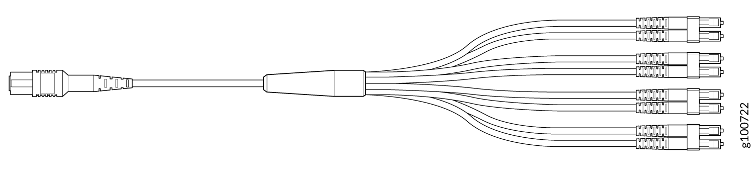
Table 3 describes the way the fibers are connected between the MPO and LC duplex connectors. The cable signals are the same as those described in Table 1.
|
MPO Connector Pin |
LC Duplex Connector Pin |
|---|---|
|
1 |
Tx on LC Duplex 1 |
|
2 |
Tx on LC Duplex 2 |
|
3 |
Tx on LC Duplex 3 |
|
4 |
Tx on LC Duplex 4 |
|
5 |
Unused |
|
6 |
Unused |
|
7 |
Unused |
|
8 |
Unused |
|
9 |
Rx on LC Duplex 4 |
|
10 |
Rx on LC Duplex 3 |
|
11 |
Rx on LC Duplex 2 |
|
12 |
Rx on LC Duplex 1 |
12-Ribbon Patch and Breakout Cables Available from Juniper Networks
Juniper Networks sells 12-ribbon patch and breakout cables with MPO connectors that meet the requirements described earlier. You are not required to purchase cables from Juniper Networks. Table 4 describes the available cables.
|
Cable Type |
Connector Type |
Fiber Type |
Cable Length |
Juniper Model Number |
|---|---|---|---|---|
|
12-ribbon patch |
Socket MPO/PC to socket MPO/PC, key up to key up |
MMF (OM3) |
1 m |
MTP12-FF-M1M |
|
3 m |
MTP12-FF-M3M |
|||
|
5 m |
MTP12-FF-M5M |
|||
|
10 m |
MTP12-FF-M10M |
|||
|
Socket MPO/APC to socket MPO/APC, key up to key up |
SMF |
1 m |
MTP12-FF-S1M |
|
|
3 m |
MTP12-FF-S3M |
|||
|
5 m |
MTP12-FF-S5M |
|||
|
10 m |
MTP12-FF-S10M |
|||
|
12-ribbon breakout |
Socket MPO/PC, key up, to four LC/UPC duplex |
MMF (OM3) |
1 m |
MTP-4LC-M1M |
|
3 m |
MTP-4LC-M3M |
|||
|
5 m |
MTP-4LC-M5M |
|||
|
10 m |
MTP-4LC-M10M |
|||
|
Socket MPO/APC, key up, to four LC/UPC duplex |
SMF |
1 m |
MTP-4LC-S1M |
|
|
3 m |
MTP-4LC-S3M |
|||
|
5 m |
MTP-4LC-S5M |
|||
|
10 m |
MTP-4LC-S10M |
24-Fiber MPO Connectors
You can use patch cables with 24-fiber MPO connectors to connect two supported transceivers of the same type—for example, 2x100GE-SR-to-2x100GE-SR.
Figure 2 shows the 24-fiber MPO optical lane assignments.
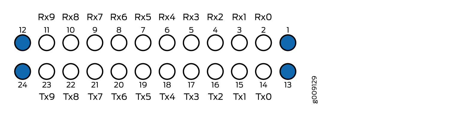
You must order cables with the correct polarity. Vendors refer to these crossover cables as key up to key up, latch up to latch up, Type B, or Method B. If you are using patch panels between two transceivers, ensure that the proper polarity is maintained through the cable plant.
The MPO optical connector for the CFP2-100G-SR10-D3 is defined in Section 5.6 of the CFP2 Hardware Specification and Section 88.10.3 of IEEE STD 802.3-2012. These specifications include the following requirements:
-
Recommended Option A in IEEE STD 802.3-2012.
-
The transceiver receptacle is a plug. A patch cable with a socket connector is required to connect to the module.
-
Ferrule finish must be a flat-polished interface that is compliant with IEC 61754-7.
-
Alignment key is key up.
The optical interface must meet the FT-1435-CORE requirement in Generic Requirements for Multi-Fiber Optical Connectors. The module must pass the wiggle test defined by IEC 62150-3.
CS Connector
You can use patch cables with CS connectors to connect two supported transceivers of the same type- for example, 2x100G-LR4 to 2x100G-LR4 or 2x100G-CWDM4 to 2x100G-CWDM4. CS connectors are compact connectors that are designed for next-generation QSFP-DD transceivers. The CS connector provides easy backward compatibility with QSFP28 and QSFP56 transceivers.
LC Duplex Connectors
You can use patch cables with LC duplex connectors to connect two supported transceivers of the same type—for example, 40GBASE-LR4-to-40GBASE-LR4 or 100GBASE-LR4-to 100GBASE-LR4. A patch cable is one fiber pair with two LC duplex connectors at opposite ends. LC duplex connectors are also used with 12-fiber ribbon breakout cables.
Figure 3 shows how to install an LC duplex connector in a transceiver.
Calculate Power Budget and Power Margin for Fiber-Optic Cables
Use the information in this topic and the specifications for your optical interface to calculate the power budget and power margin for fiber-optic cables.
You can use the Hardware Compatibility Tool page to find information about the pluggable transceivers supported on your Juniper Networks device.
To calculate the power budget and power margin, perform the following tasks:
Calculate Power Budget for Fiber-Optic Cables
To ensure that fiber-optic connections have sufficient power for correct operation, you need to calculate the link's power budget (PB), which is the maximum amount of power it can transmit. When you calculate the power budget, you use a worst-case analysis to provide a margin of error, even though all the parts of an actual system do not operate at the worst-case levels. To calculate the worst-case estimate of PB, you assume minimum transmitter power (PT) and minimum receiver sensitivity (PR):
PB = PT – PR
The following hypothetical power budget equation uses values measured in decibels (dB) and decibels referred to one milliwatt (dBm):
PB = PT – PR
PB = –15 dBm – (–28 dBm)
PB = 13 dB
How to Calculate Power Margin for Fiber-Optic Cables
After calculating a link's PB, you can calculate the power margin (PM), which represents the amount of power available after subtracting attenuation or link loss (LL) from the PB. A worst-case estimate of PM assumes maximum LL:
PM = PB – LL
PM greater than zero indicates that the power budget is sufficient to operate the receiver.
Factors that can cause link loss include higher-order mode losses, modal and chromatic dispersion, connectors, splices, and fiber attenuation. Table 5 lists an estimated amount of loss for the factors used in the following sample calculations. For information about the actual amount of signal loss caused by equipment and other factors, refer to vendor documentation.
Link-Loss Factor |
Estimated Link-Loss Value |
|---|---|
Higher-order mode losses |
Single mode—None Multimode—0.5 dB |
Modal and chromatic dispersion |
Single mode—None Multimode—None, if product of bandwidth and distance is less than 500 MHz-km |
Faulty connector |
0.5 dB |
Splice |
0.5 dB |
Fiber attenuation |
Single mode—0.5 dB/km Multimode—1 dB/km |
The following sample calculation for a 2-km-long multimode link with a PB of 13 dB uses the estimated values from Table 5. This example calculates LL as the sum of fiber attenuation (2 km @ 1 dB/km, or 2 dB) and loss for five connectors (0.5 dB per connector, or 2.5 dB) and two splices (0.5 dB per splice, or 1 dB) as well as higher-order mode losses (0.5 dB). The PM is calculated as follows:
PM = PB – LL
PM = 13 dB – 2 km (1 dB/km) – 5 (0.5 dB) – 2 (0.5 dB) – 0.5 dB
PM = 13 dB – 2 dB – 2.5 dB – 1 dB – 0.5 dB
PM = 7 dB
The following sample calculation for an 8-km-long single-mode link with a PB of 13 dB uses the estimated values from Table 5. This example calculates LL as the sum of fiber attenuation (8 km @ 0.5 dB/km, or 4 dB) and loss for seven connectors (0.5 dB per connector, or 3.5 dB). The PM is calculated as follows:
PM = PB – LL
PM = 13 dB – 8 km (0.5 dB/km) – 7(0.5 dB)
PM = 13 dB – 4 dB – 3.5 dB
PM = 5.5 dB
In both the examples, the calculated PM is greater than zero, indicating that the link has sufficient power for transmission and does not exceed the maximum receiver input power.
Fiber-Optic Cable Signal Loss, Attenuation, and Dispersion
- Signal Loss in Multimode and Single-Mode Fiber-Optic Cable
- Attenuation and Dispersion in Fiber-Optic Cable
Signal Loss in Multimode and Single-Mode Fiber-Optic Cable
Multimode fiber is large enough in diameter to allow rays of light to reflect internally (bounce off the walls of the fiber). Interfaces with multimode optics typically use LEDs as light sources. However, LEDs are not coherent sources. They spray varying wavelengths of light into the multimode fiber, which reflects the light at different angles. Light rays travel in jagged lines through a multimode fiber, causing signal dispersion. When light traveling in the fiber core radiates into the fiber cladding, higher-order mode loss results. Together these factors limit the transmission distance of multimode fiber compared with single-mode fiber.
Single-mode fiber is so small in diameter that rays of light can reflect internally through one layer only. Interfaces with single-mode optics use lasers as light sources. Lasers generate a single wavelength of light, which travels in a straight line through the single-mode fiber. Compared with multimode fiber, single-mode fiber has a higher bandwidth and can carry signals for longer distances.
Exceeding the maximum transmission distances can result in significant signal loss, which causes unreliable transmission.
Attenuation and Dispersion in Fiber-Optic Cable
Correct functioning of an optical data link depends on modulated light reaching the receiver with enough power to be demodulated correctly. Attenuation is the reduction in power of the light signal as it is transmitted. Attenuation is caused by passive media components such as cables, cable splices, and connectors. Although attenuation is significantly lower for optical fiber than for other media, it still occurs in both multimode and single-mode transmission. An efficient optical data link must have enough light available to overcome attenuation.
Dispersion is the spreading of the signal over time. The following two types of dispersion can affect an optical data link:
Chromatic dispersion—Spreading of the signal over time, resulting from the different speeds of light rays.
Modal dispersion—Spreading of the signal over time, resulting from the different propagation modes in the fiber.
For multimode transmission, modal dispersion—rather than chromatic dispersion or attenuation—usually limits the maximum bit rate and link length. For single-mode transmission, modal dispersion is not a factor. However, at higher bit rates and over longer distances, chromatic dispersion rather than modal dispersion limits maximum link length.
An efficient optical data link must have enough light to exceed the minimum power that the receiver requires to operate within its specifications. In addition, the total dispersion must be less than the limits specified for the type of link in Telcordia Technologies document GR-253-CORE (Section 4.3) and International Telecommunications Union (ITU) document G.957.
When chromatic dispersion is at the maximum allowed, its effect can be considered as a power penalty in the power budget. The optical power budget must allow for the sum of component attenuation, power penalties (including those from dispersion), and a safety margin for unexpected losses.