Contrail Services

This chapter looks at Kubernetes service in the Contrail environment. Specifically, it will focus on clusterIP and loadbalancer type of services that are commonly used in practice. Contrail uses its loadbalancer object to implement these two type of services. First, we’ll review the concept of legacy Contrail neutron load balancer, then we’ll look into the extended ECMP load balancer object, which is the object that these two types of services are based on in Contrail. The final part of this chapter explores how the clusterIP and loadbalancer service works, in detail, each with a test case built in the book’s testbed.

Kubernetes Service

Service is the core object in Kubernetes. In Chapter 3 you learned what Kubernetes service is and how to create a service object with a YAML file. Functionally, a service is running as a Layer 4 (transport layer) load balancer that is sitting between clients and servers. Clients can be anything requesting a service. The server in our context is the backend pods responding to the request. The client only sees the frontend - a service IP and service port exposed by the service, and it does not (and does not need to) care about which backend pods (and what pod IP) actually responds to the service request. Inside of the cluster, that service IP, also called cluster IP, is a kind of virtual IP (VIP).

In the Contrail environment it is implemented through floating IP.

Note

This design model is very powerful and efficient in the sense that it covers the fragility of the possible single point failure that may be caused by failure of any individual pod providing the service, therefore making a service much more robust from client’s perspective.

In the Contrail Kubernetes integrated environment, all three types of services are supported:

clusterIP
nodePort
loadbalancer

Now let’s see how the service is implemented in Contrail.

Contrail Service

Chapter 3 introduced Kubernetes’ default implementation of service through kube-proxy. In Chapter 3 we mentioned that CNI providers can have their own implementations. Well, in Contrail, nodePort service is implemented by kube-proxy. However, clusterIP and loadbalancer services are implemented by Contrail’s loadbalancer (LB).

Before diving into the details of Kubernetes service in Contrail, let’s review the legacy OpenStack-based load balancer concept in Contrail.

Tip

For brevity, sometimes loadbalancer is also referred to as LB.

Contrail Openstack Load Balancer

Contrail load balancer is a foundation feature supported since its first release. It enables the creation of a pool of VMs serving applications, sharing one virtual-ip (VIP) as the front-end IP towards clients. Figure 1 illustrates Contrail load balancer and its components.

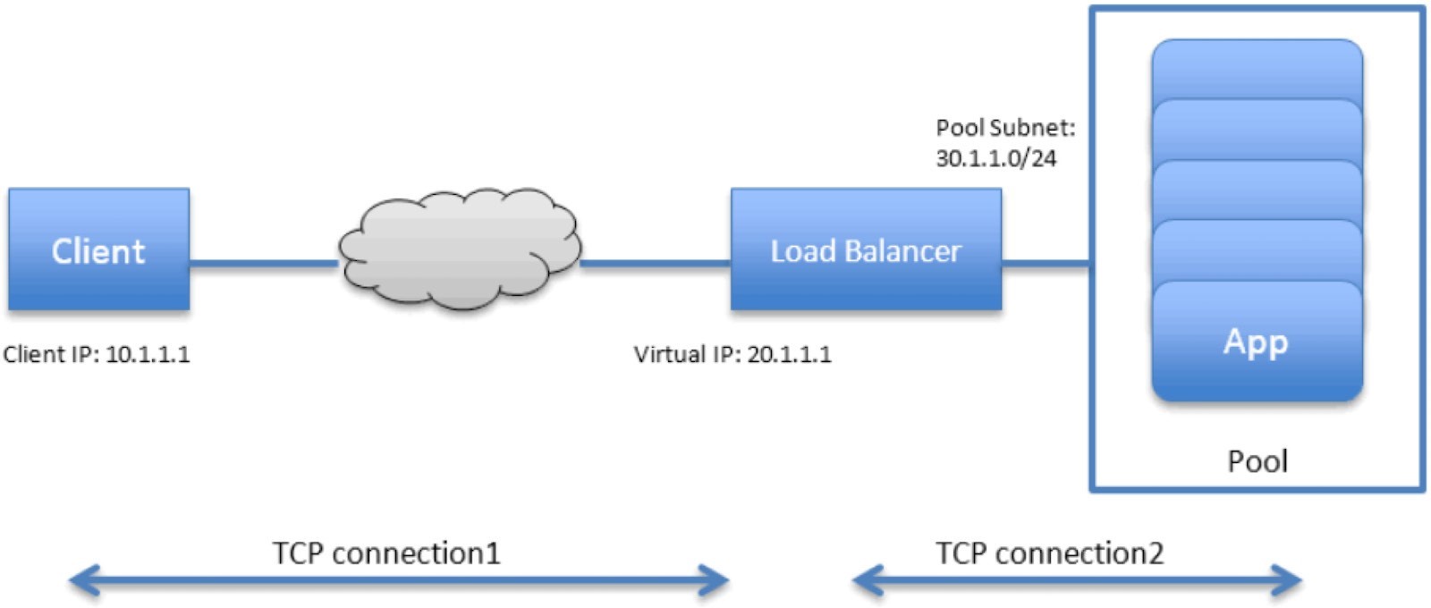
Some highlights of Figure 1 are:

The LB is created with an internal VIP 30.1.1.1. An LB listener is also created for each listening port.
Together, all back-end VMs compose a pool which is with subnet 30.1.1.0/24, the same as LB’s internal VIP.
Each back-end VM in the pool, also called a member, is allocated an IP from the pool subnet 30.1.1.0/24.
To expose the LB to the external world, it has allocated another VIP which is external VIP 20.1.1.1.
A client only sees one external VIP 20.1.1.1, representing the whole service.
When LB sees a request coming from the client, it does TCP connection proxying. That means it establishes the TCP connection with the client, extracts the client’s HTTP/HTTPS requests, creates a new TCP connection towards one of the back-end VMs from the pool, and sends the request in the new TCP connection.
When LB gets its response from the VM, it forwards the response to the client.
And when the client closes the connection to the LB, the LB may also close its connection with the back-end VM.

Tip

When the client closes its connection to the LB, the LB may or may not close its connection to the back-end VM. Depending on the performance, or other considerations, it may use a timeout before it tears down the session.

You can see that this load balancer model is very similar to the Kubernetes service concept:

VIP is the service IP.
backend VM becomes backend pods.
members are added by Kubernetes instead of OpenStack.

In fact, Contrail re-uses a good part of this model in its Kubernetes service implementation. To support service load balancing, Contrail extends the load balancer with a new driver. Along with the driver, service will be implemented as an equal cost multiple path (ECMP) load balancer working in Layer 4 (transport layer). This is the primary difference when compared with the proxy mode used by the OpenStack load balancer type.

Actually any load balancer can be integrated with Contrail via the Contrail component conrail-svc-monitor.
Each load balancer has a load balancer driver that is registered to Contrail with a loadbalancer_provider type.
The contrail-svc-monitor listens to Contrail loadbalancer, listener, pool, and member objects. It also calls the registered load balancer driver to do other necessary jobs based on the loadbalancer_provider type.
Contrail by default provides ECMP load balancer (loadbalancer_provider is native) and haproxy load balancer (loadbalancer_provider is opencontrail).
The OpenStack load balancer is using haproxy load balancer.
Ingress, on the other hand, is conceptually even closer to the OpenStack load balancer in the sense that both are Layer 7 (Application Layer) proxy-based. More about ingress will be discussed in later sections.

Contrail Service Load Balancer

Let’s take a look at service load balancer and related objects.

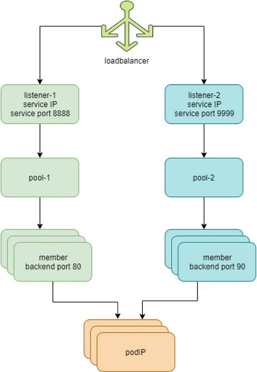
The highlights in Figure 2 are:

Each service is represented by a loadbalancer object.
The load balancer object comes with a loadbalancer_provider property. For service implementation, a new loadbalancer_provider type called native is implemented.
For each service port a listener object is created for the same service loadbalancer.
For each listener there will be a pool object.
The pool contains members, depending on the number of back-end pods, one pool may have multiple members.
Each member object in the pool will map to one of the back-end pods.
Contrail-kube-manager listens kube-apiserver for k8s service and when a custerIP or loadbalancer type of service is created, a loadbalancer object with loadbalancer_provider property native is created.
Loadbalancer will have a virtual IP VIP, which is the same as the serviceIP.
The service-ip/VIP will be linked to the interface of each back-end pod. This is done with an ECMP load balancer driver.
The linkage from service-ip to the interfaces of multiple back-end pods creates an ECMP next-hop in Contrail, and traffic will be load balanced from the source pod towards one of the back-end pods directly. Later we’ll show the ECMP prefix in the pod’s VRF table.
The contrail-kube-manager continues to listen to kube-apiserver for any changes, based on the pod list in Endpoints, it will know the most current back-end pods, and update members in the pool.

The most important thing to understand in Figure 2, as mentioned before, is that in contrast to the legacy neutron load balancer (and the ingress load balancer which we’ll discuss later), there is no application layer proxy in this process. Contrail service implementation is based on Layer 4 (transport layer) ECMP-based load balancing.

Contrail Load Balancer Objects

We’ve talked a lot about the Contrail load balancer object and you may wonder what exactly it looks like. Well it’s time to dig a little bit deeper to look at the load balancers and the supporting objects: listener, pool, and members.

In a Contrail setup you can pull the object data either from Contrail UI, CLI (curl), or third-party UI tools based on REST API. In production, depending on which one is available and handy, you can select your favorite.

Let’s explore load balancer object with curl. With the curl tool you just need a FQDN of the URL pointing to the object.

For example, to find the load balancer object URL for the service service-web-clusterip from load balancers list:

Now with one specific load balancer URL, you can pull the specific LB object details:

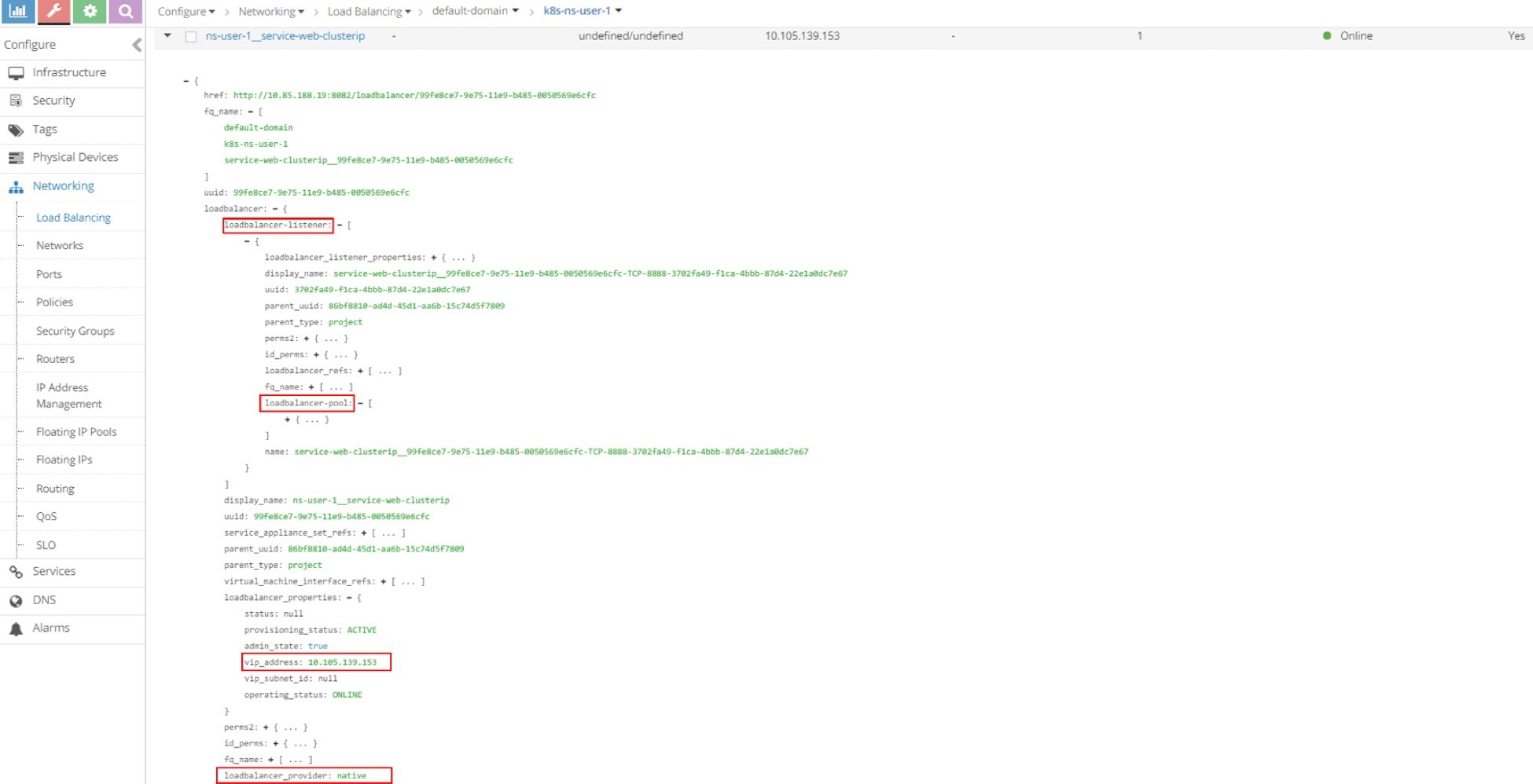
The output is very extensive and includes many details that are not of interest to us at the moment, except for a few details worth mentioning:

In loadbalancer_properties, the LB use service IP as its VIP.
The LB is connected to a listener by a reference.
The loadbalancer_provider attribute is native, a new extension to implement Layer 4 (transport layer) ECMP for Kubernetes service.

In the rest of the exploration of LB and its related objects, let’s use the legacy Contrail UI.

Tip

You can also easily use the new Contrail Command UI to do the same.

For each service there is an LB object, in Figure 3 the screen capture shows two LB objects:

ns-user-1-service-web-clusterip
ns-user-1-service-web-clusterip-mp

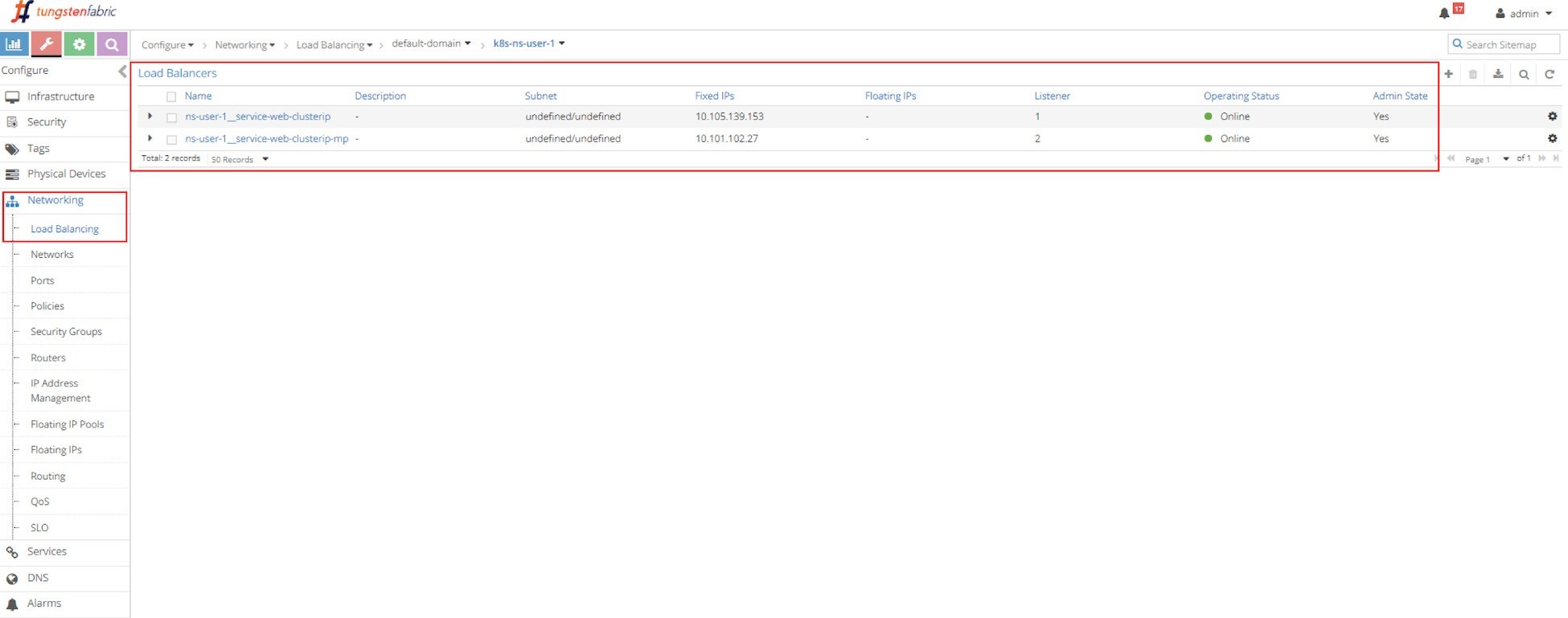
This indicates two services were created. The service load balancer object’s name is composed by connecting the NS name with the service name, hence you can tell the names of the two services:

service-web-clusterip
service-web-clusterip-mp

Click on the small triangle icon in the left of the first load balancer object ns-user-1-service-web-clusterip to expand it, then click on advanced json view icon on the right, and you will see detailed information similar to what you’ve seen in curl capture. For example, the VIP, load balancer_provider, load balancer_listener object that refers it, etc.

From here you can keep expanding the loadbalancer_listener object by clicking the + character to see the detail as shown in Figure 4. You’ll then see a loadbalancer_pool; expand it again and you will see member. You can repeat this process to explore the object data.

Listener

Click on the LB name and select listener, then expand it and display the details with JSON format and you will get the listener details. The listener is listening on service port 8888, and it is referenced by a pool in Figure 5.

Tip

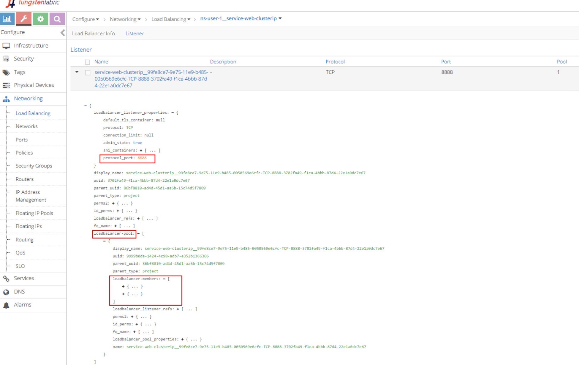
In order to see the detailed parameters of an object in JSON format, click the triangle in the left of the load balancer name to expand it, then click on the Advanced JSON view icon on the upper right corner in the expanded view. The JSON view is used a lot in this book to explore different Contrail objects.

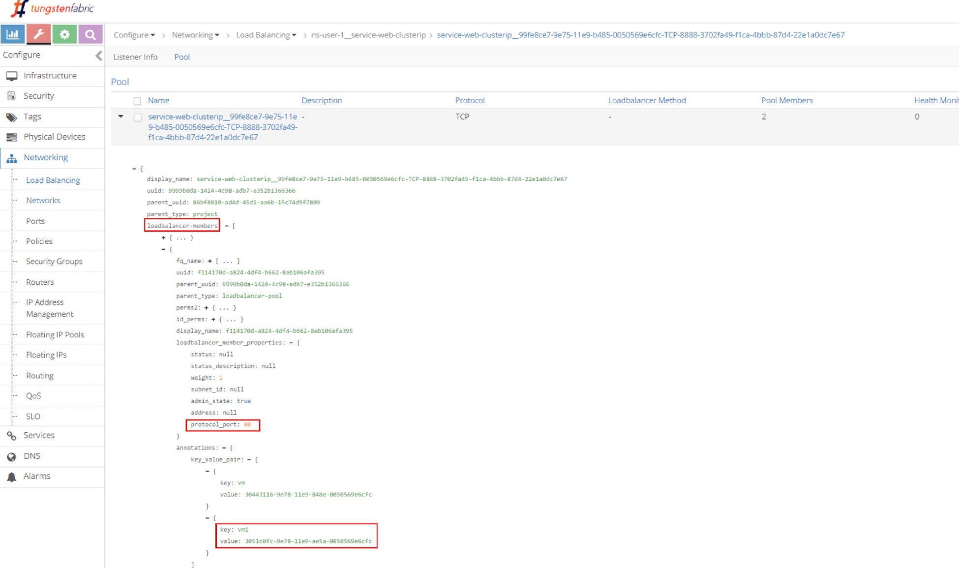
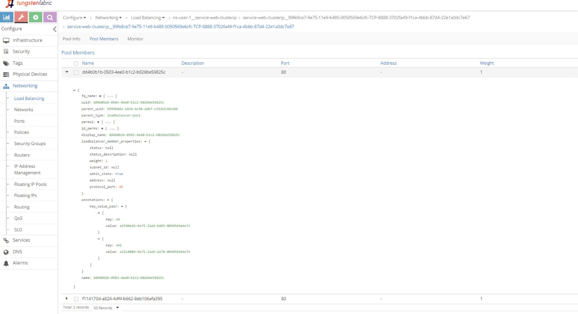
Pool and Member

Just repeating this explorative process will get you down to the pool and the two members in it. The member is with a port of 80, which maps to the container targetPort in pod as shown in Figure 6 and Figure 7.

Next we’ll examine the vRouter VRF table for the pod to show Contrail service load balancer ECMP operation details. To better understand the 1-to-N mapping between load balancer and listener shown in the load balancer object figure, we’ll also give an example of a multiple port service in our setup. We’ll conclude the clusterIP service section by inspecting the vRouter flow table to illustrate the service packet workflow.

Contrail Service Setup

Before starting our investigation, let’s look at the setup. In this book we built a setup including the following devices, most of our case studies are based on it:

one centos server running as k8s master and Contrail Controllers
two centos servers, each running as a k8s node and Contrail vRouter
one Juniper QFX switch running as the underlay leaf
one Juniper MX router running as a gateway router, or a spine
one centos server running as an Internet host machine

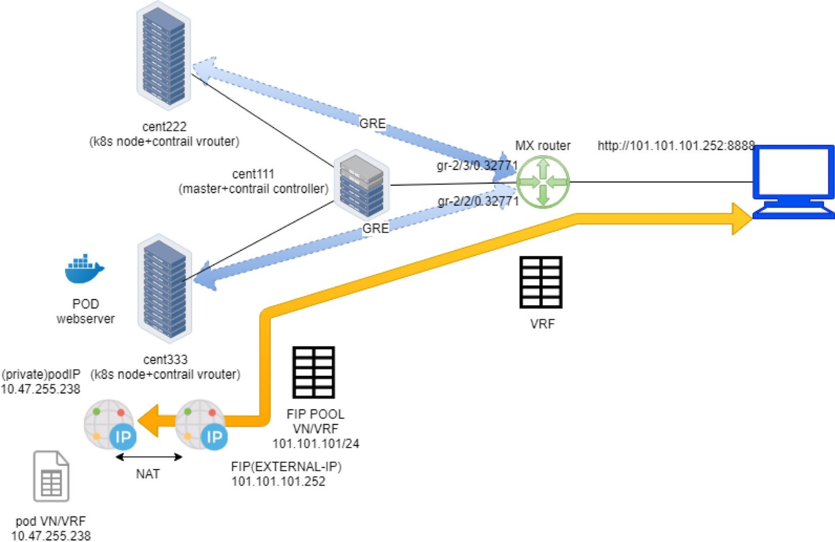
Figure 8 depicts the setup.

Note

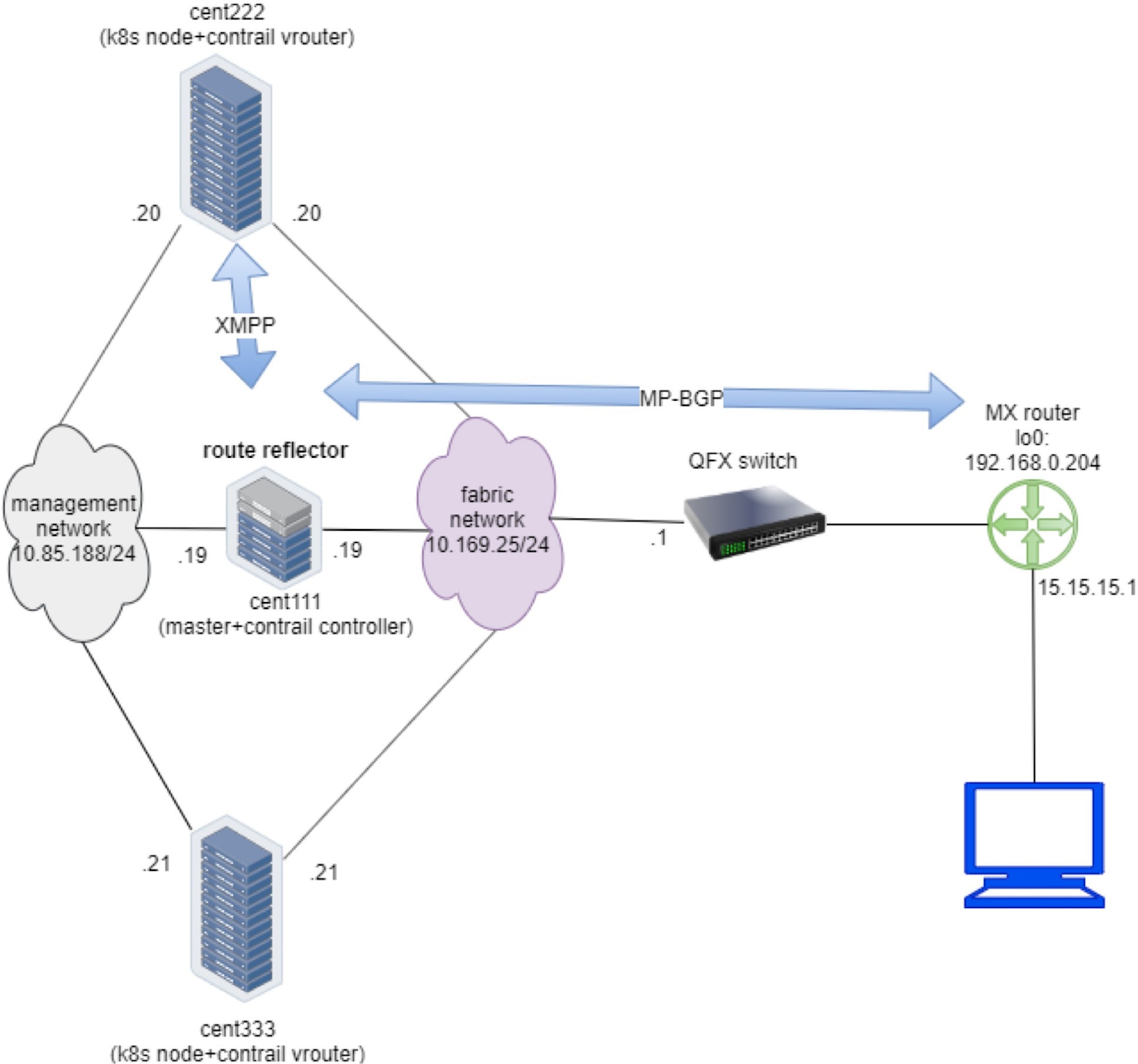
To minimize the resource utilization, all servers are actually centos VMs created by a VMware ESXI hypervisor running in one physical HP server. This is also the same testbed for ingress. The Appendix of this book has details about the setup.

Contrail ClusterIP Service

Chapter 3 demonstrated how to create and verify a clusterIP service. This section revisits the lab to look at some important details about Contrail’s specific implementations. Let’s continue on and add a few more tests to illustrate the Contrail service load balancer implementation details.

ClusterIP as Floating IP

Here is the YAML file used to create a clusterIP service:

And here’s a review of what we got from the service lab in Chapter 3:

You can see one service is created, with one pod running as its backend. The label in the pod matches the SELECTOR in service. The pod name also indicates this is a deploy-generated pod. Later we can scale the deploy for the ECMP case study, but for now let’s stick to one pod and examine the clusterIP implementation details.

In Contrail, a ClusterIP is essentially implemented in the form of a floating IP. Once a service is created, a floating IP will be allocated from the service subnet and associated to all the back-end pod VMIs to form the ECMP load balancing. Now all the back-end pods can be reached via cluserIP (along with the pod IP). This clusterIP (floating IP) is acting as a VIP to the client pods inside of the cluster.

Tip

Why does Contrail choose floating IP to implement clusterIP? In the previous section, you learned that Contrail does NAT for floating IP and service also needs NAT. So, it is natural to use the floating IP for lusterIP.

For load balancer type of service, Contrail will allocate a second floating IP - the EXTERNAL-IP as the VIP, and the external VIP is advertised outside of the cluster through the gateway router. You will get more details about these later.

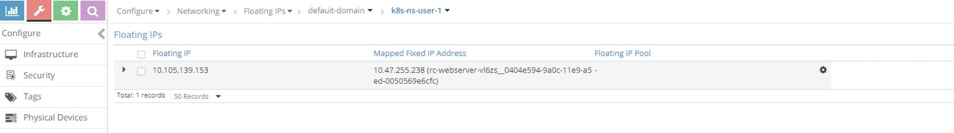
From the UI you can see the automatically allocated floating IP as lusterIP in Figure 9.

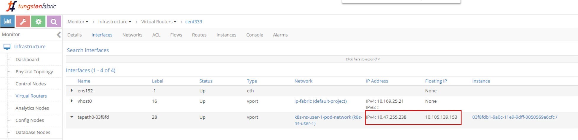
And the floating IP is also associated with the pod VMI and pod IP, in this case the VMI is representing the pod interface shown in Figure 10.

The interface can be expanded to display more details as in the next screen capture, shown in Figure 11.

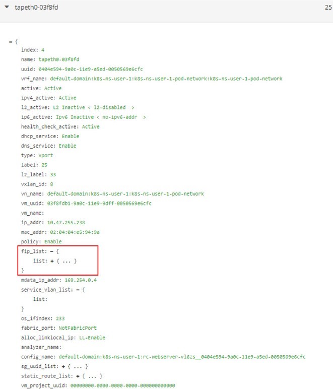
Expand the fip_list, any you’ll see the information here:

Service/clusterIP/FIP 10.105.139.153 maps to podIP/fixed_ip 10.47.255.238. The port_map says that port 8888 is a nat_port, 6 is the protocol number so it means protocol TCP. Overall, clusterIP:port 10.105.139.153:8888 will be translated to podIP:targetPort 10.47.255.238:80, and vice versa.

Now you understand with floating IP representing clusterIP, NAT will happen in service. NAT will be examined again in the flow table.

Scaling Backend Pods

In Chapter 3’s clusterIP service example, we created a service and a backend pod. To verify the ECMP, let’s increase the replica unit to 2 to generate a second backend pod. This is a more realistic model: each of the pods will now be backing each other up to avoid a single point failure.

Instead of using a YAML file to manually create a new webserver pod, with the Kubernetes spirit in mind, think of scale to a deployment, as was done earlier in this book. In our service example we’ve been using a deployment object on purpose to spawn our webserver pod:

Immediately after you create a new webserver pod by scaling the deployment with replicas 2, a new pod is launched. You end up having two backend pods, one is running in the same node cent222 as the client pod, or a local node for client pod; the other one is running in the other node cent333, the remote node from client pod’s perspective. And the endpoint objects get updated to reflect the current set of backend pods behind the service.

Note

Without the -o wide option, only the first endpoint will be displayed properly.

Let’s check the floating IP again.

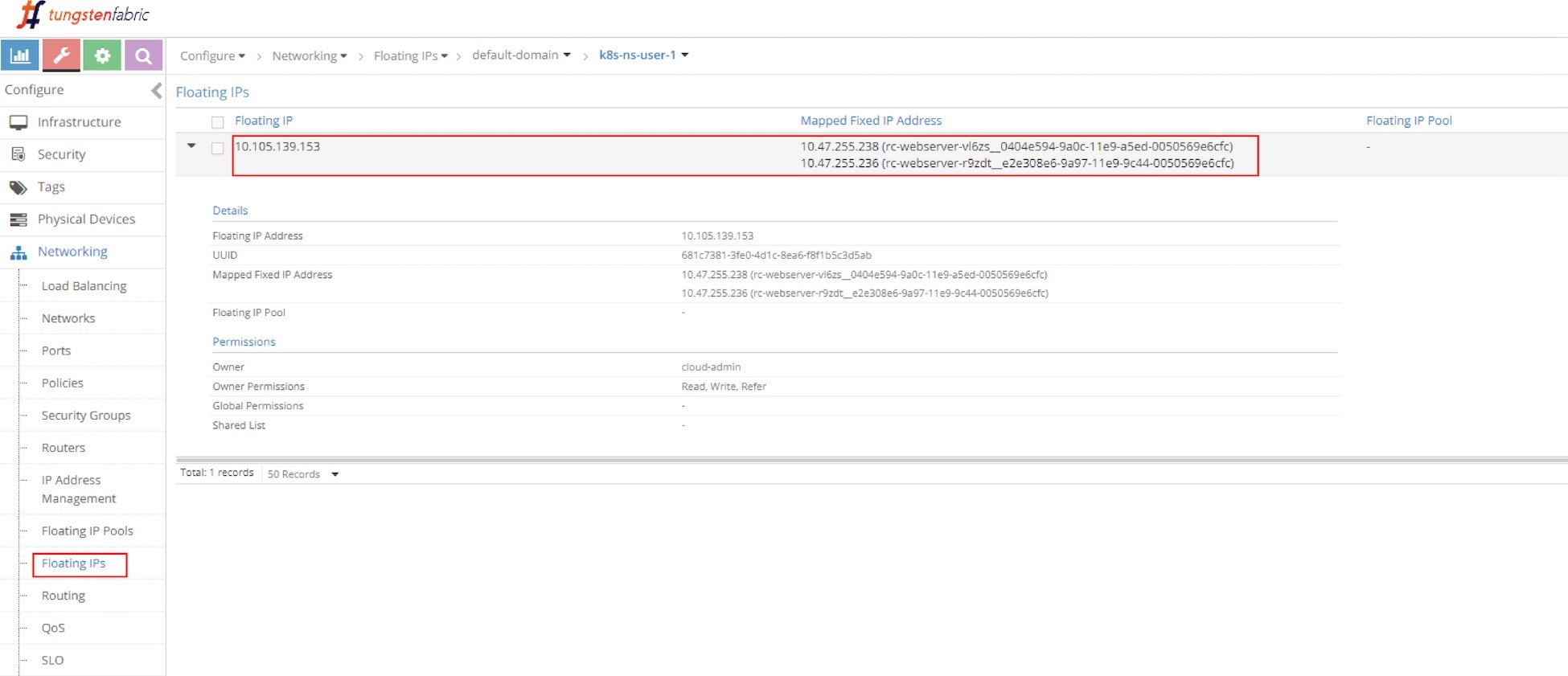
In Figure 12 you can see the same floating IP, but now it is associated with two podIPs, each representing a separate pod.

ECMP Routing Table

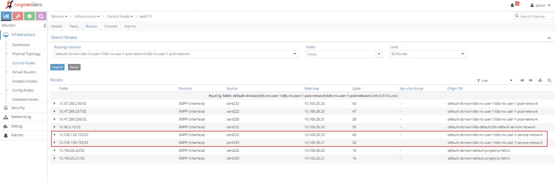
First let’s examine the ECMP. Let’s take a look at the routing table in the controller’s routing instance in the screen capture seen in Figure 13.

The routing instance (RI) has a full name with the following format:

In most cases the RI inherits the same name from its virtual network, so in this case the full IPv4 routing table has this name:

The .inet.0 indicates the routing table type is unicast IPv4. There are many other tables that are not of interest to us right now.

Two routing entries with the same exact prefixes of the clusterIP show up in the routing table, with two different next hops, each pointing to a different node. This gives us a hint about the route propagation process: both nodes (compute) have advertised the same clusterIP toward the master (Contrail Controller), to indicate the running backend pods are present in it. This route propagation is via XMPP. The master (Contrail Controller) then reflects the routes to all the other compute nodes.

Compute Node Perspective

Next, starting from the client pod node cent222, let’s look at the pod’s VRF table to understand how the packets are forwarded towards the backend pods in the screen capture in Figure 14.

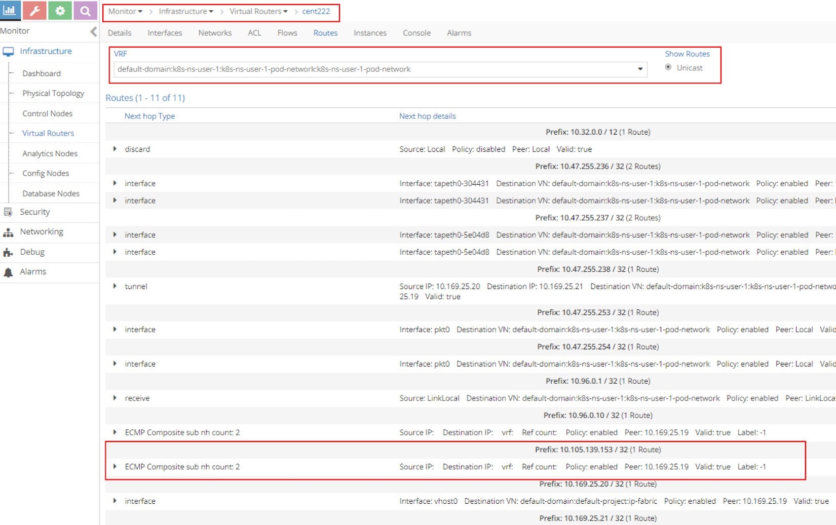
The most important part of the screenshot in Figure 14 is the routing entry Prefix: 10.105.139.153 / 32 (1 Route), as it is our clusterIP address. Underneath the prefix there is the statement ECMP Composite sub nh count: 2. This indicates the prefix has multiple possible next hops to reach.

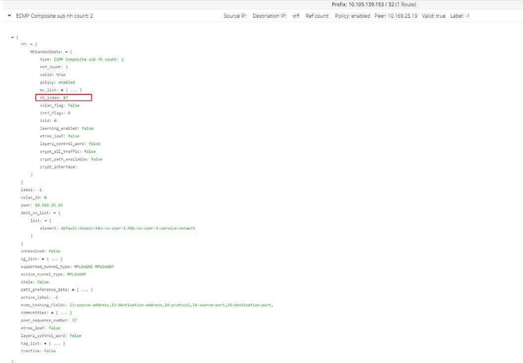
Now, expand the ECMP statement by clicking on the small triangle icon in the left and you will be given a lot more details about this prefix as shown in the next screen capture in Figure 15.

The most import of all the details in this output is that of our focus, nh_index: 87, which is the next hop ID (NHID) for the clusterIP prefix. From the vRouter agent Docker, you can further resolve the Composite NHID to the sub-NHs, which are the member next hops under the Composite next hop.

Tip

Don’t forget to execute the vRouter commands from the vRouter Docker container. Doing it directly from the host may not work:

Some important information to highlight from this output:

NHID 87 is an ECMP composite next hop.
The ECMP next hop contains two sub-next hops: next hop 43 and next hop 28, each represents a separate path towards the backend pods.
Next hop 51 represents a MPLSoUDP tunnel toward backend pod in the remote node, the tunnel is established from current node cent222, with source IP being local fabric IP 10.169.25.20, to the other node cent333 whose fabric IP is 10.169.25.21. If you recall where our two backend pods are located, this is the forwarding path between the two nodes.
Next hop 37 represents a local path, towards vif 0/8 (Oif:8), which is the local backend pod’s interface.

To resolve the vRouter vif interface, use the vif --get 8 command:

The output displays the corresponding local pod interface’s name, IP, etc.

ClusterIP Service Workflow

The clusterIP service’s load balancer ECMP workflow is illustrated in Figure 16.

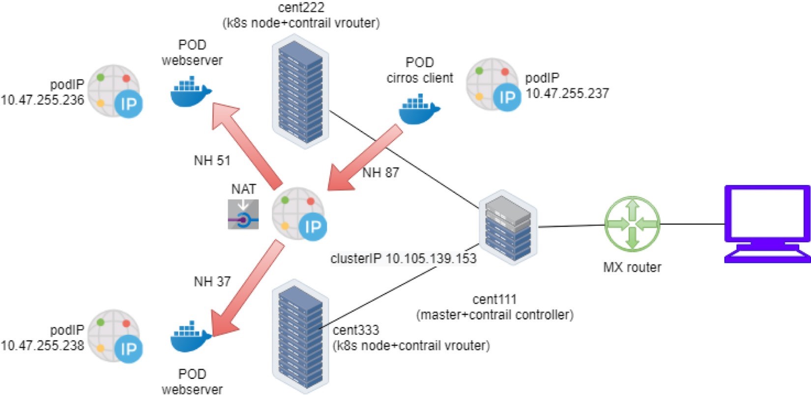
Contrail ClusterIP Service Load Balancer ECMP Forwarding

This is what happened in the forwarding plane:

A pod client located in node cent222 needs to access a service service-web-clusterip. It sends a packet towards the service’s clusterIP 10.105.139.153 and port 8888.
The pod client sends the packet to node cent222 vRouter based on the default route.
The vRouter on node cent222 gets the packet, checks its corresponding VRF table, gets a Composite next hop ID 87, which resolves to two sub-next hops 51 and 37, representing a remote and local backend pod, respectively. This indicates ECMP.
The vRouter on node cent222 starts to forward the packet to one of the pods based on its ECMP algorithm. Suppose the remote backend pod is selected, the packet will be sent through the MPLSoUDP tunnel to the remote pod on node cent333, after establishing the flow in the flow table. All subsequent packets belonging to the same flow will follow this same path. The same applies to the local path towards the local backend pod.

Multiple Port Service

You should now understand how the service Layer 4 ECMP and the LB objects in the lab work. Figure 17 shows the LB and relevant objects, and you can see that one LB may be having two or more LB listeners. Each listener has an individual backend pool that has one or multiple member(s).

In Kubernetes, this 1:N mapping between load balancer and listeners indicates a multiple port service, one service with multiple ports. Let’s look at the YAML file of it: svc/service-web-clusterip-mp.yaml:

What has been added is another item in the ports list: a new service port 9999 that maps to the container’s target- Port 90. Now, with two port mappings, you have to give each port a name, say, port1 and port2, respectively.

Note

Without a port name the multiple ports’ YAML file won’t work.

Now apply the YAML file. A new service service-web-clusterip-mp with two ports is created:

Note

To simplify the case study, the backend deployment’s replicas number has been scaled down to one.

Everything looks okay, doesn’t it? The new service comes up with two service ports exposed, 8888, the old one we’ve tested in previous examples, and the new 9999 port, should work equally well. But it turns out that is not the case. Let’s investigate.

Service port 8888 works:

Service port 9999 doesn’t work:

The request towards port 9999 is rejected. The reason is the targetPort is not running in the pod container, so there is no way to get a response from it:

The readinessProbe introduced in Chapter 3 is the official Kubernetes tool to detect this situation, so in case the pod is not ready, it will be restarted and you will catch the events.

To resolve this let’s start a new server in the pod to listen on a new port 90. One of the easiest ways to start a HTTP server is to use the SimpleHTTPServer module that comes with the python package. In this test we only need to set its listening port to 90 (the default value is 8080):

The targetPort is on. Now you can again start the request towards service port 9999 from the cirros pod. This time it succeeds and gets the returned webpage from Python’s SimpleHTTPServer:

Next, for each incoming request, the SimpleHTTPServer logs one line of output with an IP address showing where the request came from. In this case, the request is coming from the client pod with the IP address:

Contrail Flow Table

So far, we’ve tested the clusterIP service and we’ve seen client requests are sent towards the service IP. In Contrail, vrouter is the module that does all of the packet forwarding. When the vrouter gets a packet from the client pod, it looks up the corresponding VRF table in the vRouter module for the client pod (client), gets the next hop, and resolves the correct egress interface and proper encapsulation. So far, the client and backend pods are in two different nodes, and the source vrouter decides the packets needed to be sent in the MPLSoUDP tunnel, towards the node where the backend pod is running. What interests us the most?

How are the service IP and backend pod IP translated to each other?
Is there a way to capture and see the two IPs in a flow, before and after the translations, for comparison purposes?

The most straightforward method you would think of is to capture the packets, decode, and then see the results. Doing that, however, may not be as easy as what you expect. First you need to capture the packet at different places:

At the pod interface, this is after the address is translated, and that’s easy.
At the fabric interface, this is before packet is translated and reaches the pod interface. Here the packets are with MPLSoUDP encapsulation since data plane packets are tunneled between nodes.

Then you need to copy the pcap file out and load with Wireshark to decode. You probably also need to configure Wireshark to recognize the MPLSoUDP encapsulation.

An easier way to do this is to check the vRouter flow table, which records IP and port details about a traffic flow. Let’s test it by preparing a big file, file.txt, in the backend webserver pod and try to download it from the client pod.

Tip

You may wonder: in order to trigger a flow why we don’t simply use the same curl test to pull the webpage? That’s what we did in an early test. In theory, that is fine. The only problem is that the TCP flow follows the TCP session. In our previous test with curl, the TCP session starts and stops immediately after the webpage is retrieved, then the vRouter clears the flow right away. You won’t be fast enough to capture the flow table at the right moment. Instead, downloading a big file will hold the TCP session – as long as the file transfer is ongoing the session will remain – and you can take time to investigate the flow. Later on, the Ingress section will demonstrate a different method with a one-line shell script.

So, in the client pod curl URL, instead of just giving the root path / to list the files in folder, let’s try to pull the file: file.txt:

And in the server pod we see the log indicating the file downloading starts:

Now, with the file transfer going on, there’s enough time to collect the flow table from both the client and server nodes, in the vRouter container:

Client node flow table:

Highlights in this output are:

The client pod starts the TCP connection from its pod IP 10.47.255.237 and a random source port, towards the service IP 10.101.102.27 and server port 9999.
The flow TCP flag SSrEEr indicates the session is established bi-directionally.
The Action: F means forwarding. Note that there is no special processing like NAT happening here.

Note

When using a filter such as --match 15.15.15.2 only flow entries with Internet Host IPs are displayed.

We can conclude, from the client node’s perspective, that it only sees the service IP and is not aware of any backend pod IP at all.

Let’s look at the server node flow table in the server node vRouter Docker container:

Look at the second flow entry first – the IPs look the same as the one we just saw in the client side capture. Traffic lands the vRouter fabric interface from the remote client pod node, across the MPLSoUDP tunnel. Destination IP and the port are service IP and the service port, respectively. Nothing special here.

However, the flow Action is now set to N(DPd), not F. According to the header lines in the flow command output, this means NAT, or specifically, DNAT (Destination address translation) with DPAT (Destination port translation) – both the service IP and service port are translated to the backend pod IP and port.

Now look at the first flow entry. The source IP 10.47.255.238 is the backend pod IP and the source port is the Python server port 90 opened in backend container. Obviously, this is returning traffic indicating the downloading of the file is still ongoing. The Action is also NAT(N), but this time it is the reverse operation – source NAT (SNAT) and source PAT(SPAT).

The vRouter will translate the backend’s source IP source port to the service IP and port, before putting it into the MPLSoUDP tunnel and returning back to the client pod in remote node.

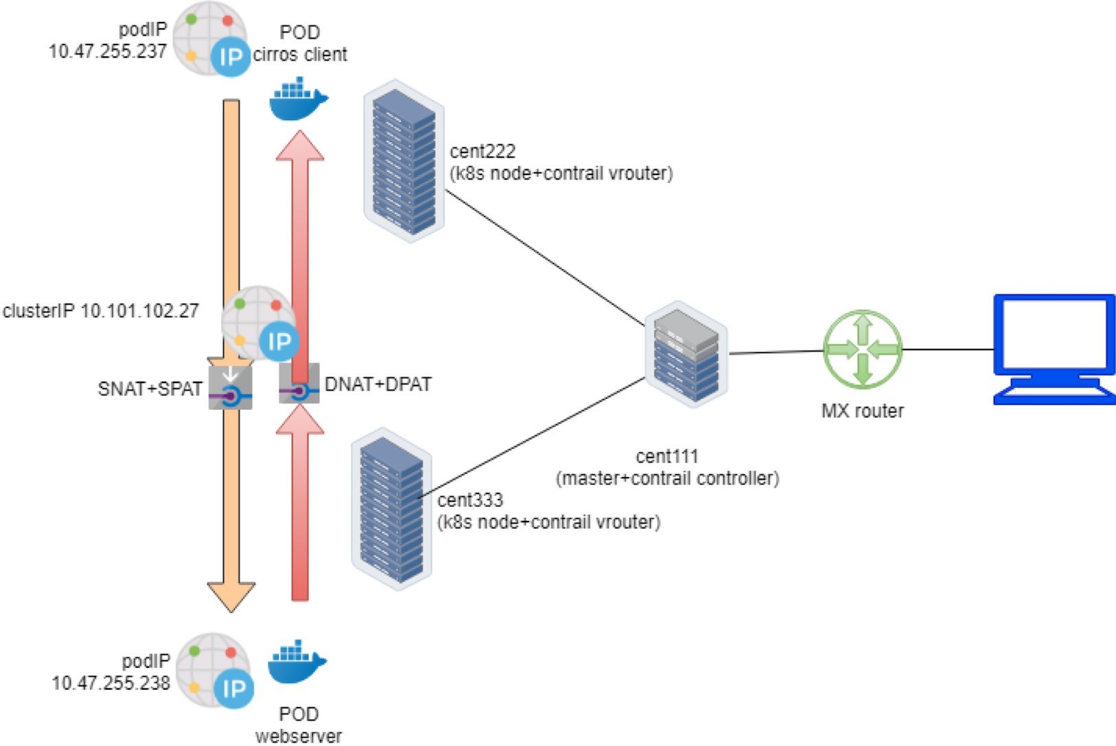
The complete end-to-end traffic flow is illustrated in Figure 18.

Contrail Load Balancer Service

Chapter 3 briefly discussed load balancer service. It mentioned that if the goal is to expose the service to the external world outside of the cluster, then just specify ServiceType as the LoadBalancer in the service YAML file.

In Contrail, whenever a service of type: LoadBalancer gets created, not only will a clusterIP be allocated and exposed to other pods within the cluster, but also a floating IP from the public floating IP pool will be assigned to the load balancer instance as an external IP and exposed to the public world outside of the cluster.

While the clusterIP is still acting as a VIP to the client inside of the cluster, the floating ip or external ip will essentially act as a VIP facing those clients sitting outside of the cluster, for example, a remote Internet host which sends requests to the service across the gateway router.

The next section demonstrates how the LoadBalancer type of service works in our end-to-end lab setup, which includes the Kubernetes cluster, fabric switch, gateway router, and Internet host.

External IP as Floating IP

Let’s look at the YAML file of a LoadBalancer service. It’s the same as the clusterIP service except just one more line declaring the service type:

Create and verify the service:

Compare the output with the clusterIP service type, this time there is an IP allocated in the EXTERNAL-IP column. If you remember what we’ve covered in the floating IP pool section, you should understand this EXTERNAL-IP is actually another FIP, allocated from the NS FIP pool or global FIP pool. We did not give any specific floating IP pool information in the service object YAML file, so based on the algorithm the right floating IP pool will be used automatically.

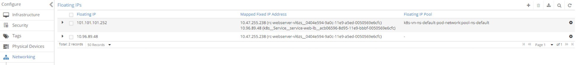
From the UI you can see that for the loadbalancer service we now have two floating IPs: one as a clusterIP (internal VIP) and the other one as EXTERNAL-IP (external VIP), as can be seem in Figure 19:

Two Floating IPs for a Load Balancer Service

Both floating IPs are associated with the pod interface shown in the next screen capture, Figure 20.

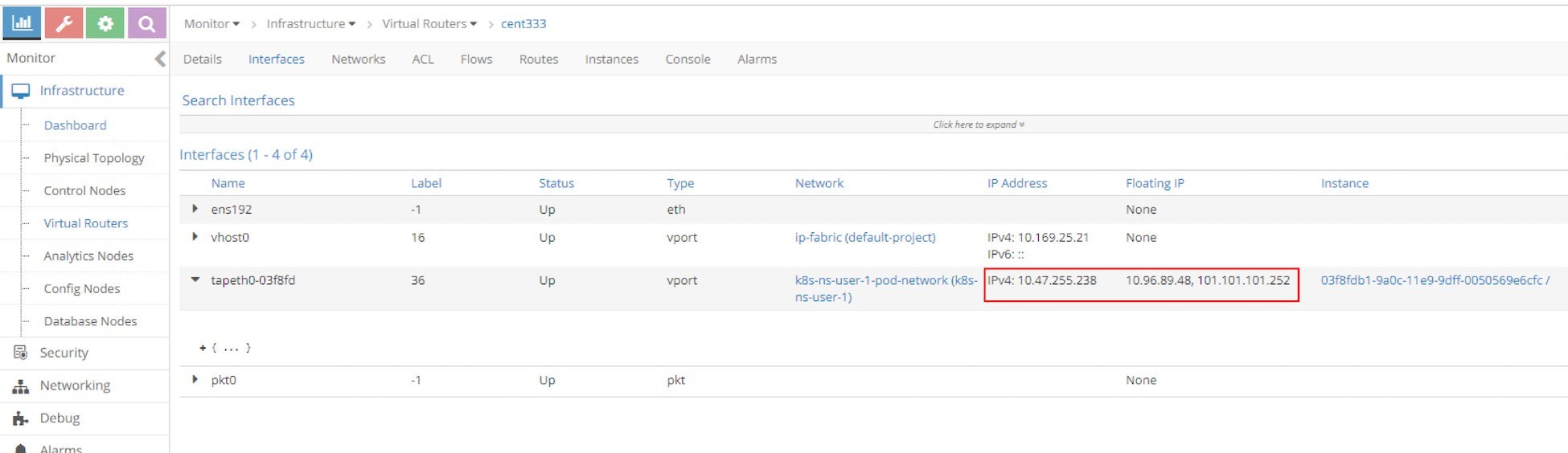
Expand the tap interface and you will see two floating IPs listed in the fip_list:

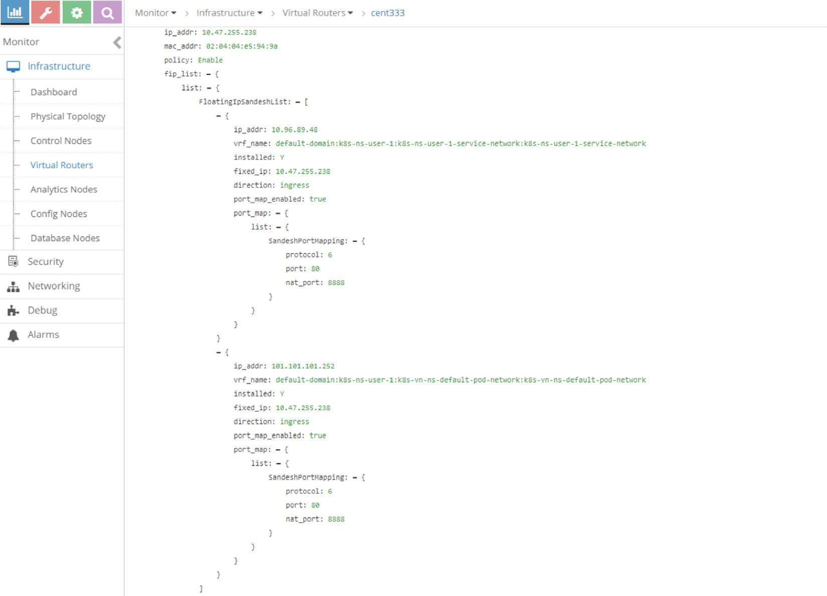
Now you should understand the only difference here between the two types of services is that for the load balancer service, an extra FIP is allocated from the public FIP pool, which is advertised to the gateway router and acts as the outside-facing VIP. That is how the loadbalancer service exposes itself to the external world.

Gateway Router VRF Table

In the Contrail floating IP section you’ve learned how to advertise floating IP. But now let’s review the main concepts to understand how it works in Contrail service implementation.

The route-target community setting in the floating IP VN makes it reachable by the Internet host, so effectively our service is now also exposed to the Internet instead of only to pods inside of the cluster. Examining the gateway router’s VRF table reveals this:

The floating IP host route is learned by the gateway router from the Contrail controller – more specifically, Contrail control node – which acts as a standard MP-BGP VPN RR reflecting routes between compute nodes and the gateway router. A further look at the detailed version of the same route displays more information about the process:

Highlights of the output here are:

The source indicates from which BGP peer the route is learned, 10.169.25.19 is the Contrail Controller (and Kubernetes master) in the book’s lab.
The protocol next hop tells who generates the route. And 10.169.25.20 is node cent222 where the backend webserver pod is running.
The gr-2/2/0.32771 is an interface representing the (MPLS over) GRE tunnel between the gateway router and node cent333.

Load Balancer Service Workflow

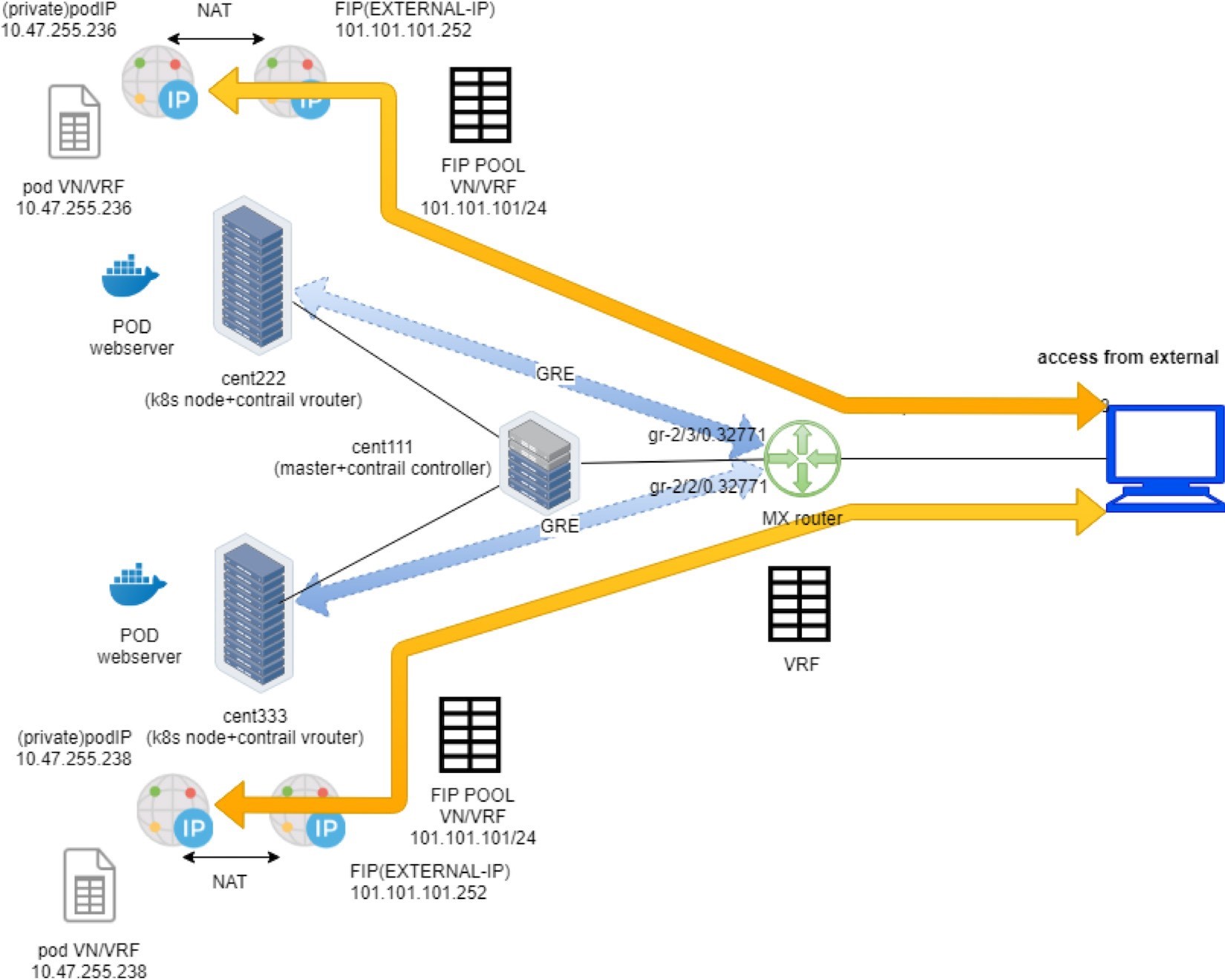
To summarize, the floating IP is given to the service as its external IP is advertised to the gateway router and gets loaded into the router’s VRF table. When the Internet host sends a request to the floating IP through the MPLSoGRE tunnel, the gateway router will forward it to the compute node where the backend pod is located.

The packet flow is illustrated in Figure 22.

Here is the full story of Figure 22:

Create a FIP pool from a public VN, with route-target. The VN is advertised to the remote gateway router via MP-BGP.
Create a pod with a label app: webserver, and Kubernetes decides the pod will be created in node cent333. The node publishes the pod IP via XMPP.
Create a loadbalancer type of service with service port and label selector app=webserver. Kubernetes allocates a service IP.
Kubernetes finds the pod with the matching label and updates the endpoint with the pod IP and port information.
Contrail creates a loadbalancer instance and assigns a floating IP to it. Contrail also associates that floating IP with the pod interface, so there will be a one-to-one NAT operation between the floating IP and the pod IP.
Via XMPP, node cent333 advertises this floating IP to Contrail Controller cent111, which then advertises it to the gateway router.
On receiving the floating IP prefix, the gateway router checks and sees that the RT of the prefix matches what it’s expecting, and it will import the prefix in the local VRF table. At this moment the gateway learns the next hop of the floating IP is cent333, so it generates a soft GRE tunnel toward cent333.
When the gateway router sees a request coming from the Internet toward the floating IP, it will send the request to the node cent333 through the MPLS over GRE tunnel.
The vRouter in the node sees the packets destined to the floating IP, it will perform NAT so the packets will be sent to the right backend pod.

Verify Load Balancer Service

To verify end-to-end service access from Internet host to the backend pod, let’s log in to the Internet host desktop and launch a browser, with URL pointing to http://101.101.101.252:8888.

Tip

Keep in mind that the Internet host request has to be sent to the public floating IP, not to the service IP (clusterIP) or backend pod IP which are only reachable from inside the cluster!

You can see the returned web page on the browser below in Figure 23.

Tip

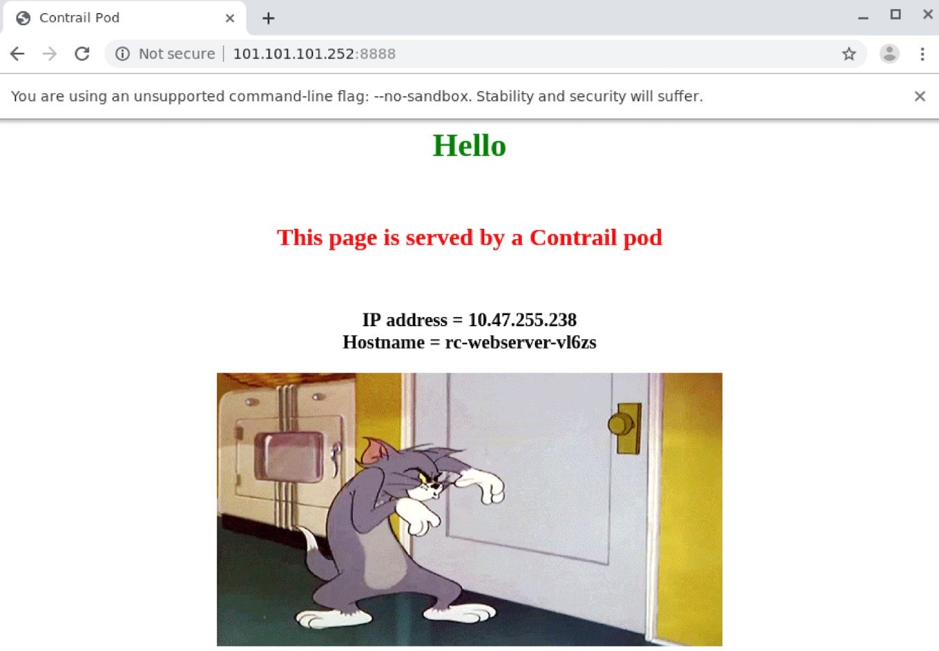
This book’s lab installed a Centos desktop as an Internet host.0

To simplify the test, you can also SSH into the Internet host and test it with the curl tool:

And the Kubernetes service is available from the Internet!

Load Balancer Service ECMP

You’ve seen how the load balancer type of service is exposed to the Internet and how the floating IP did the trick. In the clusterIP service section, you’ve also seen how the service load balancer ECMP works. But what you haven’t seen yet is how the ECMP processing works under the load balancer type of service. To demonstrate this we again scale the RC to generate one more backend pod behind the service:

Here’s the question: with two pods on different nodes, and both as backend now, from the gateway router’s perspective, when it gets the service request, which node does it choose to forward the traffic to?

Let’s check the gateway router’s VRF table again:

The same floating IP prefix is imported, as we’ve seen in the previous example, except that now the same route is learned twice and an additional MPLSoGRE tunnel is created. Previously, in the clusterIP service example, the detail option was used in the show route command to find the tunnel endpoints. This time we examine the soft GRE gr- interface to find the same:

The IP-Header of the gr- interface indicates the two end points of the GRE tunnel:

10.169.25.20:192.168.0.204: Here the tunnel is between node cent222 and the gateway router.
10.169.25.21:192.168.0.204: Here the tunnel is between node cent333 and the gateway router

We end up needing two tunnels in the gateway router, each pointing to a different node where a backend pod is running. Now we believe the router will perform ECMP load balancing between the two GRE tun- nels, whenever it gets a service request toward the same floating IP. Let’s check it out.

Verify Load Balancer Service ECMP

To verify ECMP let’s just pull the webpage a few more times and we can expect to see both pod IPs eventually displayed.

Turns out this never happens!

Tip

Lynx is another terminal web browser similar to the w3m program that we used earlier.

The only webpage is from the first backend pod 10.47.255.236, webserver-846c9ccb8b-xkjpw, running in node cent222. The other one never shows up. So the expected ECMP does not happen yet. But when you examine the routes using the detail or extensive keyword, you’ll find the root cause:

This reveals that even if the router learned the same prefix from both nodes, only one is Active and the other won’t take effect because it is NotBest. Therefore, the second route and the corresponding GRE interface gr- 2/2/0.32771 will never get loaded into the forwarding table:

This is the default Junos BGP path selection behavior, but a detailed discussion of that is beyond the scope of this book.

Note

For the Junos BGP path selection algorithm, go to the Juniper TechLibrary: https://www. juniper.net/documentation/en_US/junos/topics/topic-map/bgp-path-selection.html.

The solution is to enable the multipath vpn-unequal-cost knob under the VRF table:

Now let’s check the VRF table again:

A Multipath with both GRE interfaces will be added under the floating IP prefix, and the forwarding table reflects the same:

Now, try to pull the webpage from the Internet host multiple times with curl or a web browser and you’ll see the random result – both backend pods get the request and responses back:

The end-to-end packet flow is illustrated in Figure 24.

ON THIS PAGE

Contrail Services

Kubernetes Service

Contrail Service

Contrail Service Load Balancer

Contrail Service Setup

Contrail ClusterIP Service

Contrail Load Balancer Service