EVPN/VXLAN GPU Backend Fabric – GPU Multitenancy

GPU Multitenancy (GPU as a Service – GPUaaS)

GPU as a Service (GPUaaS) is a model where GPU compute resources are provided on demand to users or applications, similar to other utility-style computing services. Rather than dedicating entire servers or clusters to a single team or purpose, GPUaaS allows resources to be dynamically allocated based on current workload requirements. Tenants can request specific numbers of GPUs, often across multiple servers, and use them for tasks such as AI training, data analytics, or visualization. The service abstracts the underlying infrastructure, providing users with a seamless and scalable experience while maintaining secure and efficient resource isolation. By combining flexibility with centralized management, GPUaaS enables better resource utilization and simplifies operations in environments where multiple teams or projects share the same data center.

GPU multitenancy is a resource management approach that allows multiple tenants to use GPU resources independently within a shared infrastructure. Instead of assigning all the GPUs in a server to a single tenant, GPU multitenancy enables more flexible allocation, where one or more GPUs on a server can be reserved for different tenants. This model improves efficiency by allowing organizations to match GPU resources to the specific needs of each workload, rather than over-provisioning entire servers. Each tenant operates in a logically isolated environment, with clear separation of compute resources, network paths, and associated configurations. This isolation ensures that tenants can run their applications without interference, while administrators maintain centralized control over GPU distribution and access.

GPU multitenancy and GPU as a Service (GPUaaS) are closely related concepts that, when combined, enable efficient and scalable use of GPU infrastructure in multi-tenant environments. GPU multitenancy provides the foundation by allowing GPU resources to be flexibly assigned to different tenants at a granular level, whether one GPU, several GPUs, or specific GPUs across different servers. This approach ensures that each tenant operates in a logically isolated environment, maintaining security and performance consistency even when physical infrastructure is shared.

Building on this, GPUaaS abstracts these capabilities into an on-demand service model. Instead of requiring users to manage physical servers or hardware configurations, GPUaaS delivers GPU resources dynamically as needed. It leverages the underlying multitenancy framework to allocate GPUs based on user requests, enforce isolation, and optimize usage across a diverse set of workloads. This allows data centers to support a wide range of teams or applications concurrently, without dedicating entire servers to each one.

Together, GPU multitenancy and GPUaaS enable high efficiency, better resource utilization, and operational simplicity. While multitenancy handles the secure and flexible slicing of GPU resources, GPUaaS delivers these slices as consumable services, scaling compute capacity up or down as needed, and making GPU-powered computing more accessible and cost-effective for varied use cases.

Types of GPU multitenancy

SERVER ISOLATION:

In a server isolation model, each tenant is allocated one or more entire servers. All GPUs within those servers are exclusively dedicated to a single tenant, ensuring full physical and logical separation from other tenants. This model simplifies resource allocation and minimizes the risk of cross-tenant interference, making it well suited for workloads that require predictable performance and strict isolation. (Figure 4).

Figure 4: GPU as a Service – Server Isolation

GPU ISOLATION:

In a GPU isolation model, individual GPUs within a server are assigned to different tenants. This allows multiple tenants to securely share the same physical server, with each tenant accessing only the GPUs allocated to them. The underlying fabric provides logical separation and guarantees isolation at the GPU level, enabling greater flexibility and higher utilization of resources without compromising security or performance. (Figure 5).

Figure 5: GPU as a Service – GPU Isolation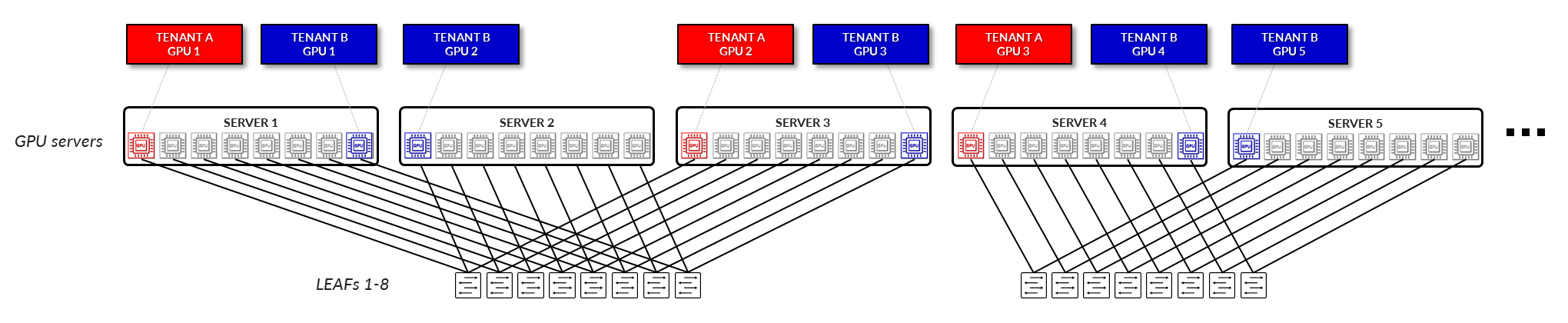

GPU Backend Fabric for Multitenancy Architecture

The design of the GPU Backend Fabric for Multitenancy follows a 3-stage Clos, rail-optimized stripe architecture using EVPN/VXLAN. This approach enables high-performance communication between GPUs assigned to the same tenant while ensuring traffic isolation between tenants, for both Server Isolation and GPU Isolation. For more information on server isolation and GPU isolation, see Rail Alignment and Local Optimization Considerations with GPU multitenancy.

Figure 6: GPU Backend Fabric Architecture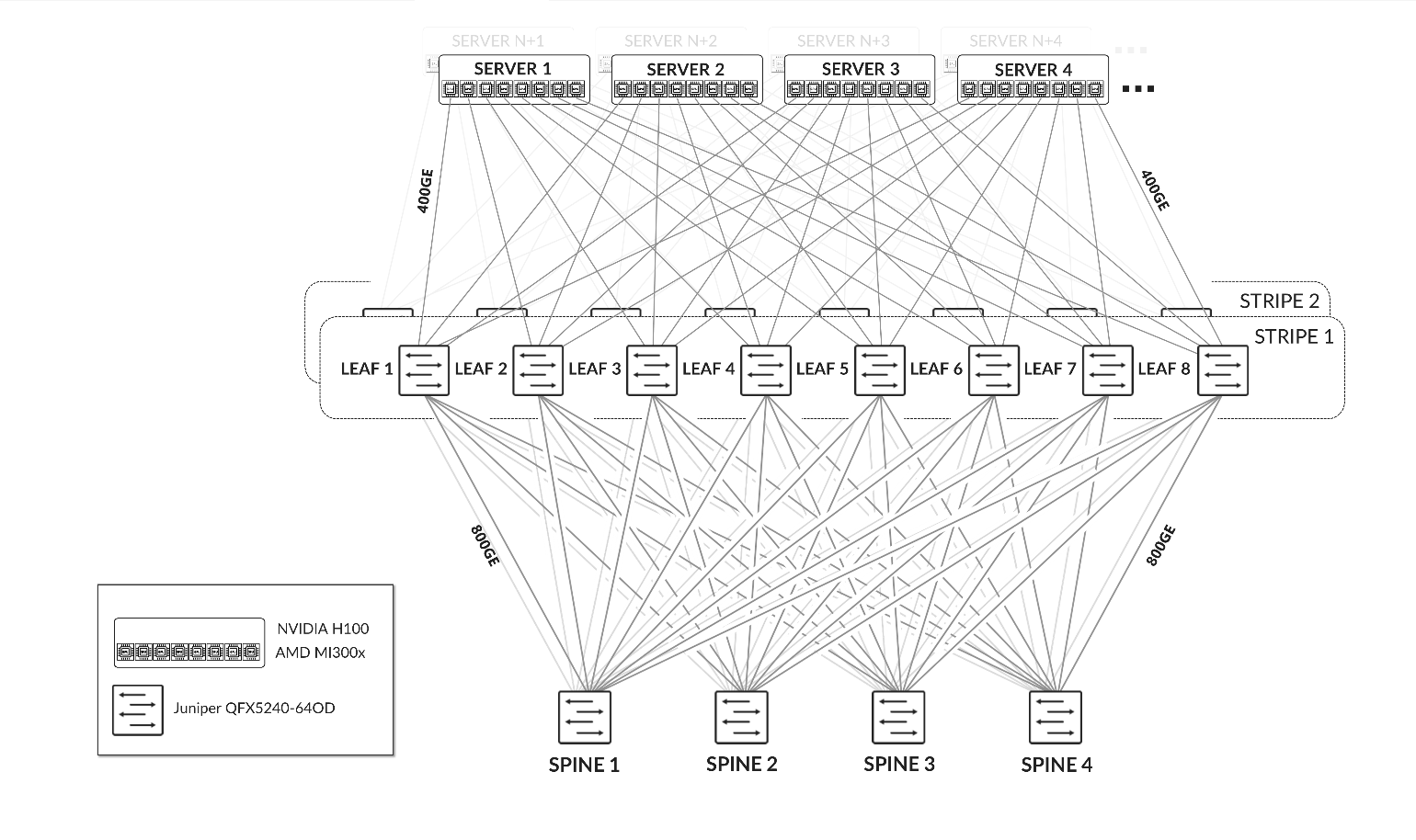

Figure 7: GPU Backend Fabric EVPN/VXLAN connectivity – Server Isolation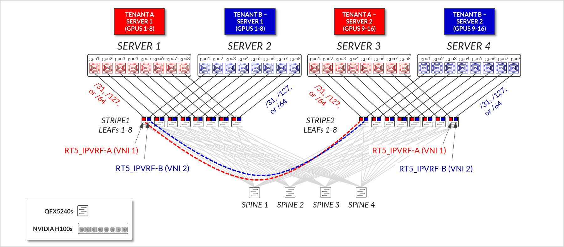

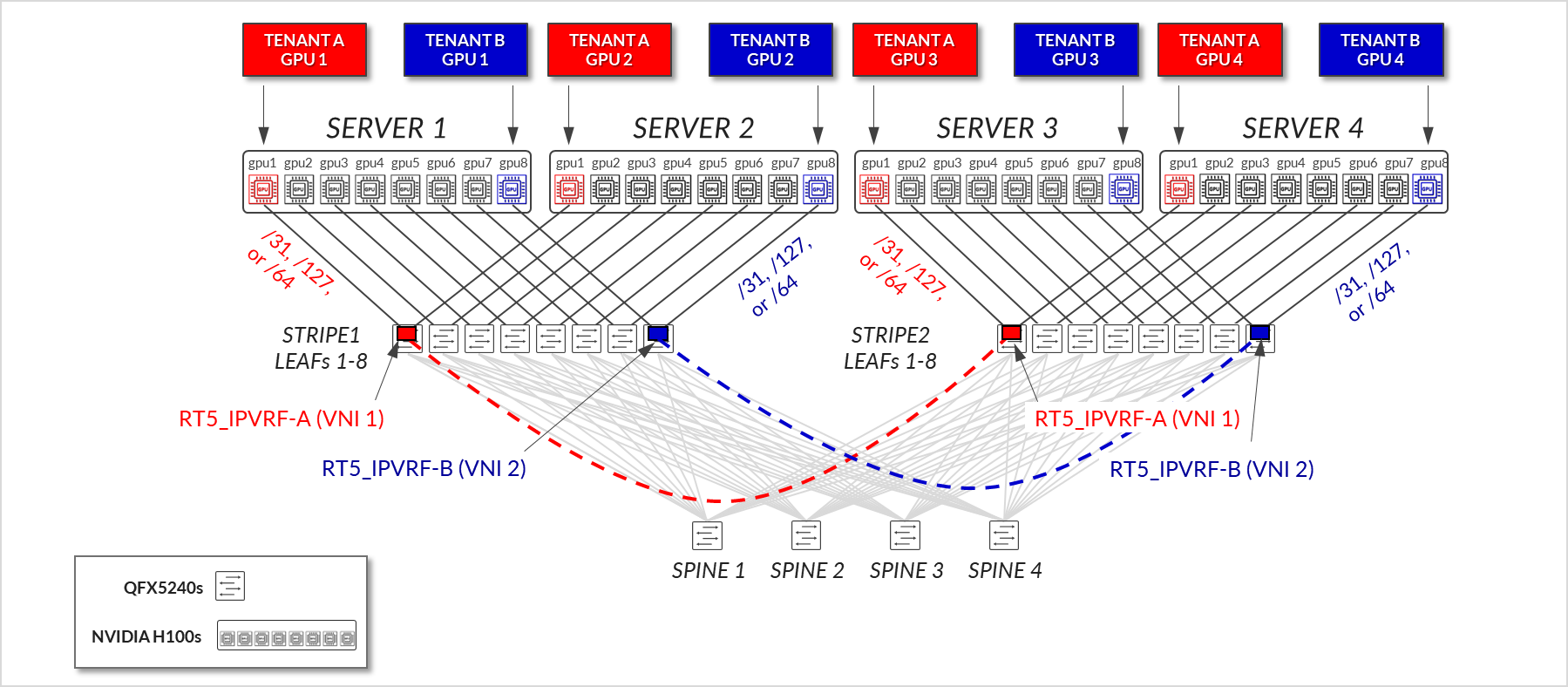
Figure 8: GPU Backend Fabric EVPN/VXLAN Connectivity – GPU Isolation

The devices that are part of the GPU Backend fabric in the AI Lab, and the connections between them, are summarized in Table 1 and Table 2:

Table 1: GPU Backend devices per Stripe

Stripe	GPU Servers	GPU Backend Leaf nodes switch model	GPU Backend Spine nodes switch model
1	MI300X x 2 (MI300X-01 & MI300X-02) H100 x 2 (H100-01 & H100-02)	QFX5240-64OD x 8 (gpu-backend-001_leaf#; #=1-8)	QFX5240-64OD x 4 (gpu-backend-spine#; #=1-4)
2	MI300X x 2 (MI300X-03 & MI300X-04) H100 x 2 (H100-01 & H100-02)	QFX5240-64OD x 8 (gpu-backend-002_leaf#; #=1-8)

All the Nvidia H100 and AMD MI300X GPU servers are connected to the GPU backend fabric using 400GE interfaces.

Table 2: GPU Backend connections between servers, leaf nodes and spine nodes.

Stripe	GPU Servers <=> GPU Backend Leaf Nodes	GPU Backend Leaf Nodes <=> GPU Backend Spine Nodes
1	Total number of 400GE links between servers and leaf nodes = 8 (number of GPUs per server) x 1 (number of 400GE server to leaf links) x 4 (number of servers) = 32	Total number of 400GE links between GPU backend leaf nodes and spine nodes = 8 (number of leaf nodes) x 2 (number of 400GE links per leaf to spine connection) x 4 (number of spine nodes) = 64
2	Total number of 400GE links between servers and leaf nodes = 8 (number of GPUs per server) x 1 (number of 400GE server to leaf links) x 4 (number of servers) = 32	Total number of 400GE links between GPU backend leaf nodes and spine nodes = 8 (number of leaf nodes) x 2 (number of 400GE links per leaf to spine connection) x 4 (number of spine nodes) = 64

The speed and number of links between the GPU servers and leaf nodes, and between the leaf and spine nodes determines the oversubscription factor. As an example, consider the number of GPU servers available in the lab, and how they are connected to the GPU backend fabric as described above.

The bandwidth between the servers and the leaf nodes is 25.6 Tbps (Table 3), while the bandwidth available between the leaf and spine nodes is also 51.2 Tbps (Table 4). This means that the fabric has enough capacity to process all traffic between the GPUs even when this traffic is 100% inter-stripe and has extra capacity to accommodate 4 more servers. With 4 additional servers the subscription factor would be 1:1 (no oversubscription).

Table 3: Per stripe Server to Leaf Bandwidth

Server to Leaf Bandwidth per Stripe
Stripe	Number of servers per Stripe	Number of 400 GE server ó leaf links per server (Same as number of leaf nodes & number of GPUs per server)	Server <=> Leaf Link Bandwidth [Gbps]	Total Servers <=> Leaf Links Bandwidth per stripe [Tbps]
1	4	8	400 Gbps	4 x 8 x 400 Gbps = 12.8 Tbps
2	4	8	400 Gbps	4 x 8 x 400 Gbps = 12.8 Tbps
			Total Server <=> Leaf Bandwidth	25.6 Tbps

Table 4: Per stripe Leaf to Spine Bandwidth

Leaf nodes to spine nodes bandwidth per Stripe
Stripe	Number of leaf nodes	Number of spine nodes	Number of 800 GE leaf ó spine links per leaf node	Server <=> Leaf Link Bandwidth [Gbps]	Bandwidth Leaf <=> Spine Per Stripe [Tbps]
1	8	4	1	800 Gbps	8 x 4 x 1 x 800 Gbps = 25.6 Tbps
2	8	4	1	800 Gbps	8 x 4 x 1 x 400 Gbps = 25.6 Tbps
				Total Leaf <=> Spine Bandwidth	51.2 Tbps

GPU to leaf nodes connectivity follows the Rail-optimized architecture as described in Backend GPU Rail Optimized Stripe Architecture.

Backend GPU Rail Optimized Stripe Architecture

A Rail Optimized Stripe Architecture provides efficient data transfer between GPUs, especially during computationally intensive tasks such as AI Large Language Models (LLM) training workloads, where seamless data transfer is necessary to complete the tasks within a reasonable timeframe. A Rail Optimized topology aims to maximize performance by providing minimal bandwidth contention, minimal latency, and minimal network interference, to provide this efficient data transfer.

In a Rail Optimized Stripe Architecture there are two important concepts: rail and stripe.

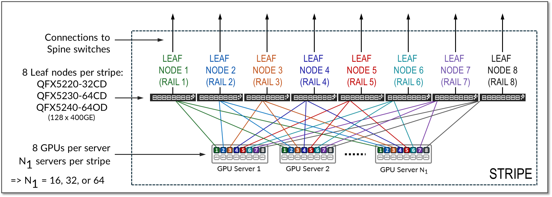
The GPUs on a server are numbered 1-8, where the number represents the GPU’s position in the server, as shown in Figure 9.

A rail connects GPUs of the same order across one of the leaf nodes in the fabric; that is, rail N connects GPUs in position N in all the servers to leaf node N.

Figure 9: Rails in a Rail Optimized Architecture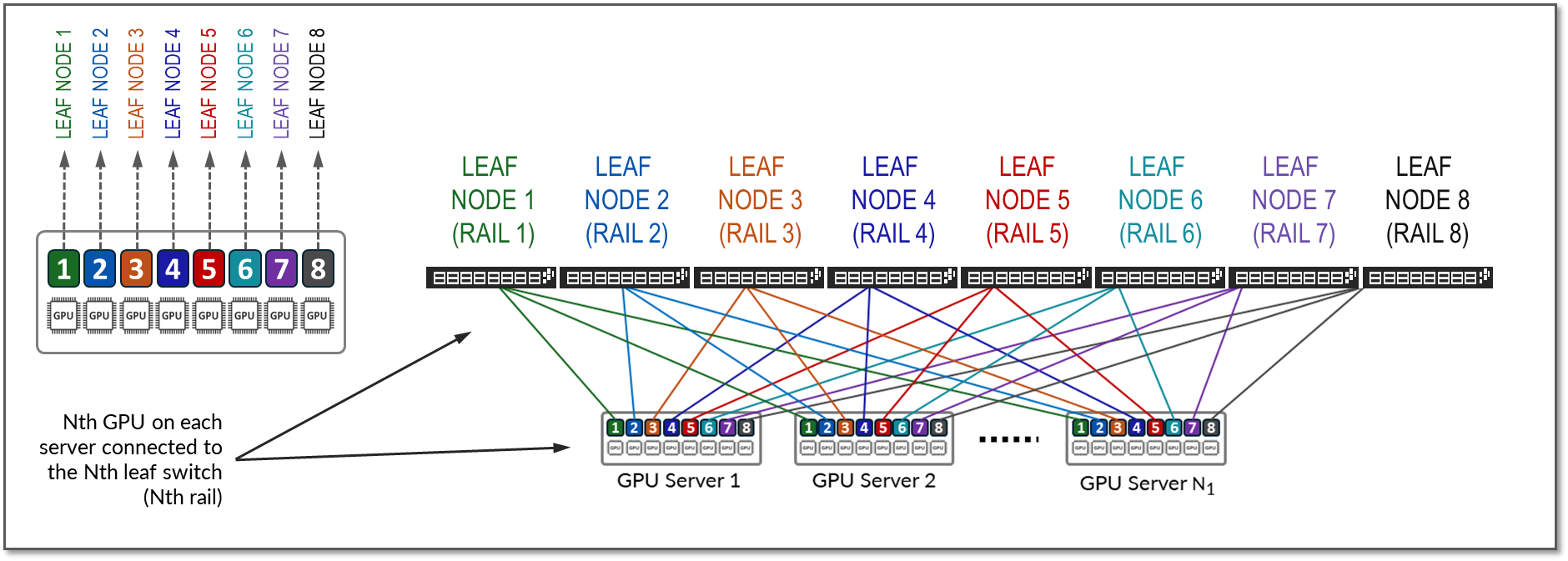

A stripe refers to a design module or building block consisting of a group of Leaf nodes and GPU servers, as shown in Figure 10. This module can be replicated to scale up the AI cluster.

Figure 10: Stripes in a Rail Optimized Architecture

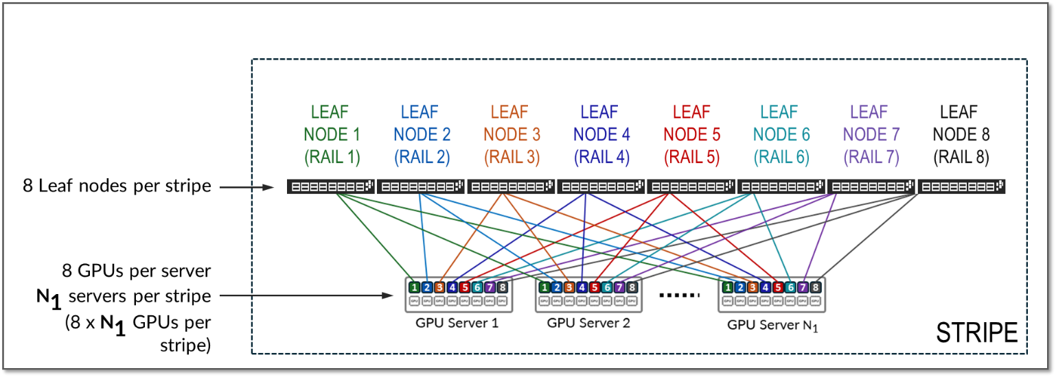
The number of leaf nodes in a single stripe, and thus the number of rails in a single stripe, is always defined by the number of GPUs per server. Each GPU server typically includes 8 GPUs. Therefore, a single stripe typically includes 8 leaf nodes (8 rails).

In a rail optimized architecture, the maximum number of servers supported in a single stripe (N1 in Figure 7) is limited by the number and the speed of the interfaces supported by the Leaf node switch model. This is because the total bandwidth between the GPU servers and leaf nodes must match the total bandwidth between leaf and spine nodes to maintain a 1:1 subscription ratio, which is ideal.

Assuming all the interfaces on the leaf node operate at the same speed, half of the interfaces will be used to connect to the GPU servers, and the other half to connect to the spines. Thus, the maximum number of servers in a stripe is calculated as half the total interfaces on each leaf node. Some examples are included in Table 5.

Table 5: Maximum number of GPUs supported per stripe

Leaf Node QFX switch Model	Maximum number of 400 GE interfaces per switch	Maximum number of servers supported per stripe (1:1 Subscription)	GPUs per server	Maximum number of GPUs supported per stripe
QFX5220-32CD	32	32 ÷ 2 = 16	8	16 servers x 8 GPUs/server = 128 GPUs
QFX5230-64CD	64	64 ÷ 2 = 32	8	32 servers x 8 GPUs/server = 256 GPUs
QFX5240-64OD	128	128 ÷ 2 = 64	8	64 servers x 8 GPUs/server = 512 GPUs

• QFX5220-32CD switches provide 32 x 400 GE ports (16 will be used to connect to the servers and 16 will be used to connect to the spine nodes)
• QFX5230-64CD switches provide up to 64 x 400 GE ports (32 will be used to connect to the servers and 32 will be used to connect to the spine nodes).
• QFX5240-64OD switches provide up to 128 x 400 GE ports (64 will be used to connect to the servers and 64 will be used to connect to the spine nodes). See Figure 11.

Note:

QFX5240-64OD switches come with 64 x 800GE ports which can break out into 2x400GE ports, for a maximum of 128 400GE interfaces was shown in table 5.

Figure 11: Maximum number of Servers per Stripes in a Rail Optimized Architecture.

As an example of how to calculate the number of servers supported, and to reinforce the concepts of rail and stripe, consider a hypothetical switch with only 8 ports of the same speed, and GPU servers with 8 GPUs each, as shown in Figure 12.

Figure 12. Number of Servers Supported by 8-Port Switches as Leaf Nodes Example.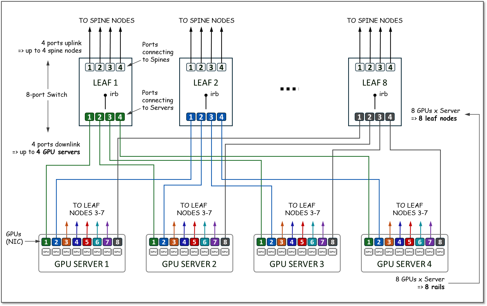

Because the GPU servers have 8 GPUs, the number of Leaf nodes will be 8. On each leaf node, 4 ports will be used to connect to the Spine Nodes (for scaling purposes as described in the next section), and 4 ports will be used to connect to the GPU servers. All the GPU numbered 1, will be connected to Leaf node 1, all the GPUs numbered 2 will be connected to Leaf node 2, and so on, with each group representing a RAIL (8 RAILS total), and the group of all 4 servers, and 8 switches together represent a STRIPE (with a total of 32 GPUs), as shown in Figure 13.

Figure 13. Stripe and Rails with 8 leaf (8-port switch) Nodes Example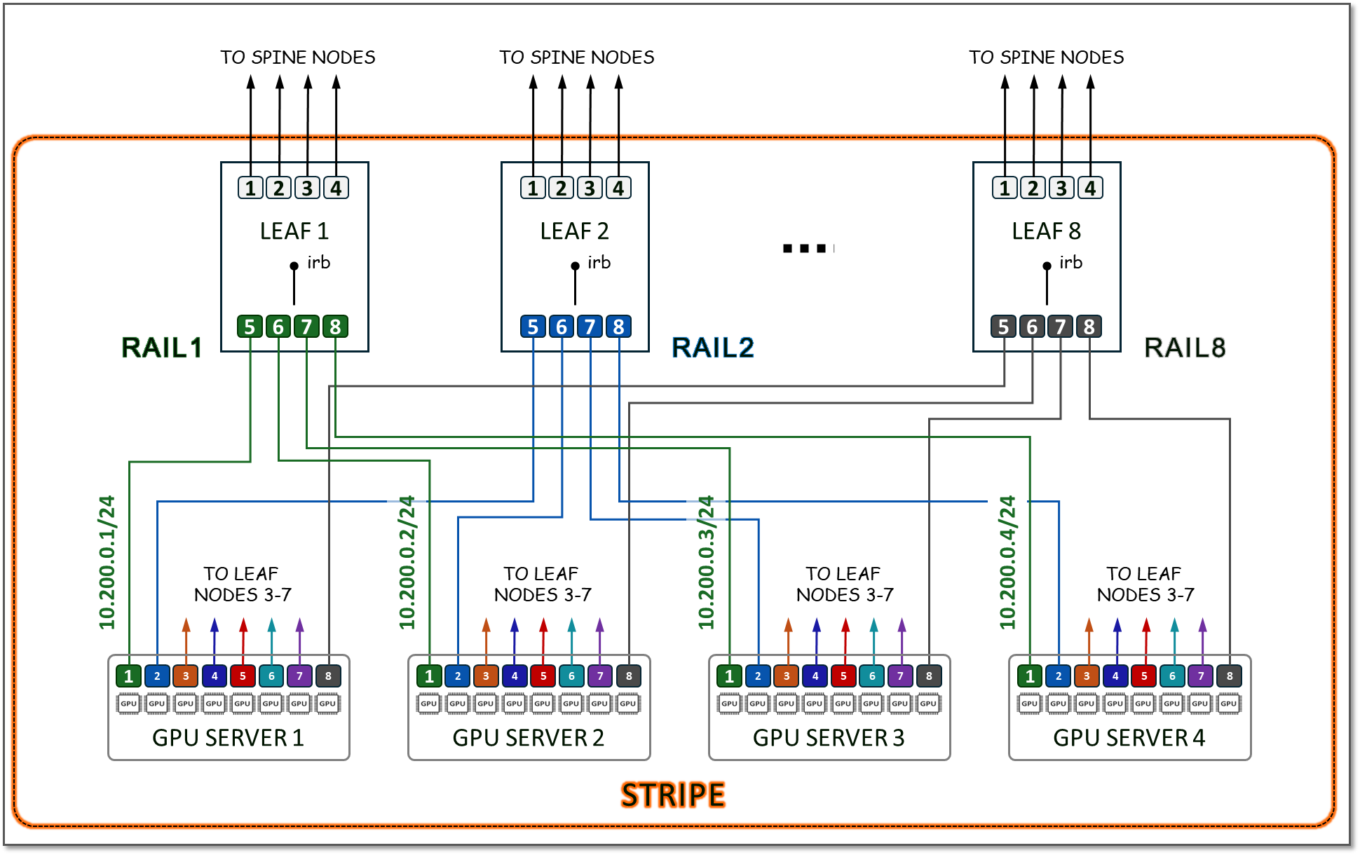

To achieve larger scales, multiple stripes can be implemented. The stripes are connected using Spine switches which provide inter-stripe connectivity, as shown in Figure 14.

Figure 14: Multiple Stripes Connected via Spine Nodes

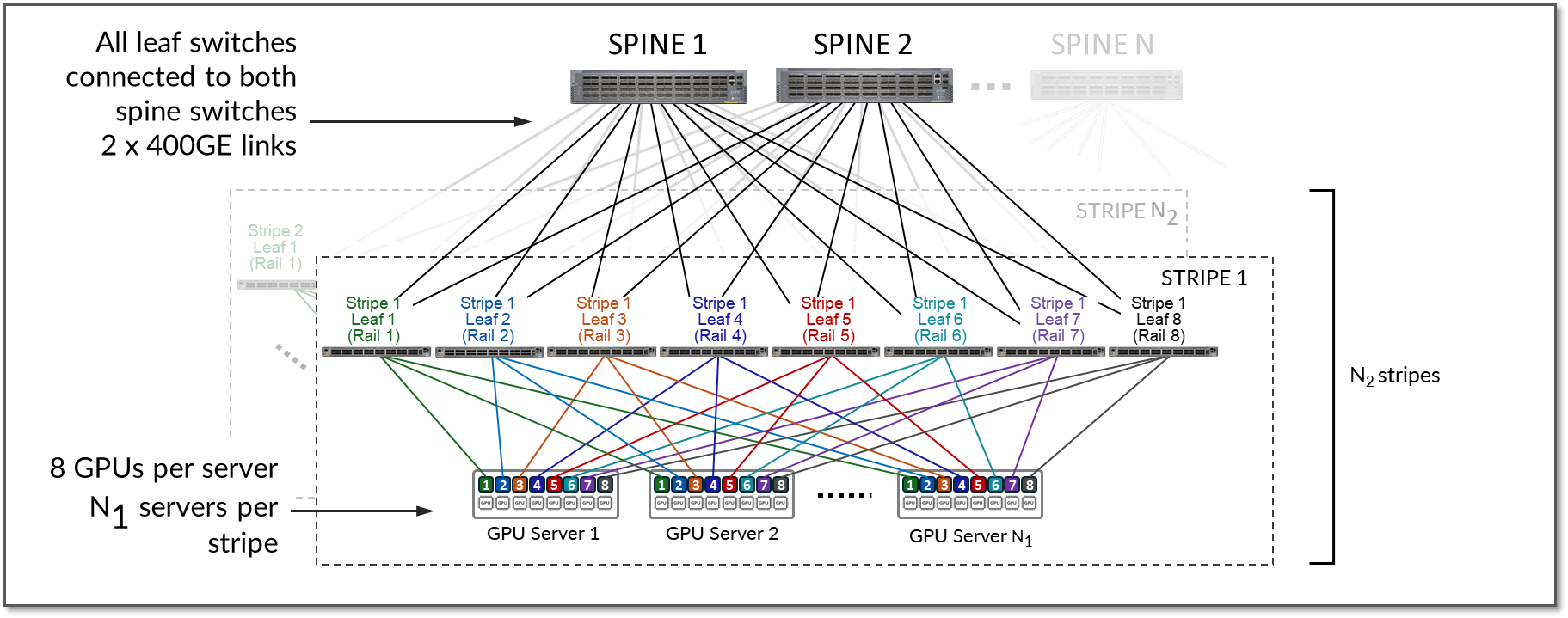
For example, assume that the desired number of GPUs is 16,000 and the fabric is using either QFX5230-64CD or QFX5240-64OD as leaf nodes:

• The QFX5240-64OD leaf nodes support up to 128 x 400Gbps ports
• The Maximum Number of Servers Per Stripe (N₁) is calculated by dividing the number of ports supported by the leaf node.

N₁ = 128 ÷ 2 = 64

• The Maximum Number of GPUs supported per stripe is calculated by multiplying the maximum number of servers per stripe (N₁) by the numbers of GPUs on each server:

N₁ x 8 = 64 x 8 = 512

• The Required Number of Stripes (N₂₎ is calculated by dividing the required number of GPUs by the maximum number of GPUs supported per stripe:

N₂ = 16000/512 ≈ 31.25 stripes (rounded up to 32)

Note:

With N₂ = 64 stripes & N₁ servers = 32, the cluster can provide 16,384 GPUs.If N₂ is increased to 72 & N₁ servers = 32, the cluster can provide 18432 GPUs.

The stripes in the AI JVD setup consist of wither 8 Juniper QFX5220-32CD, QFX5230-64CD or QFX5240-64OD switches depending on the cluster and stripe, as summarized in Table 6.

Table 6. Maximum number of GPUs supported per cluster in the JVD lab

Cluster	Stripe	Leaf Node QFX model	Maximum number of GPUs supported per stripe
1	1	QFX5230-64CD	32 servers x 8 GPUs/server = 256 GPUs
1	2	QFX5220-32CD	16 servers x 8 GPUs/server = 128 GPUs
Total number of GPUs supported by the cluster = 384 GPUs
2	1	QFX5240-64OD	64 servers x 8 GPUs/server = 512 GPUs
2	2	QFX5240-64OD	64 servers x 8 GPUs/server = 512 GPUs
Total number of GPUs supported by the cluster = 1024 GPUs

Local Optimization

Optimization in rail-optimized topologies refers to how GPU communication is managed to minimize congestion and latency while maximizing throughput. A key part of this optimization strategy is keeping traffic local whenever possible. By ensuring that GPU communication remains within the same rail or stripe or even within the same server when possible, the need to traverse spines or external links is reduced. This lowers latency, minimizes congestion, and enhances overall efficiency.

While localizing traffic is prioritized, inter-stripe communication will be necessary in larger GPU clusters. Inter-stripe communication is optimized by means of proper routing and balancing techniques over the available links to avoid bottlenecks and packet loss. The essence of optimization lies in leveraging the topology to direct traffic along the shortest and least-congested paths, ensuring consistent performance even as the network scales.

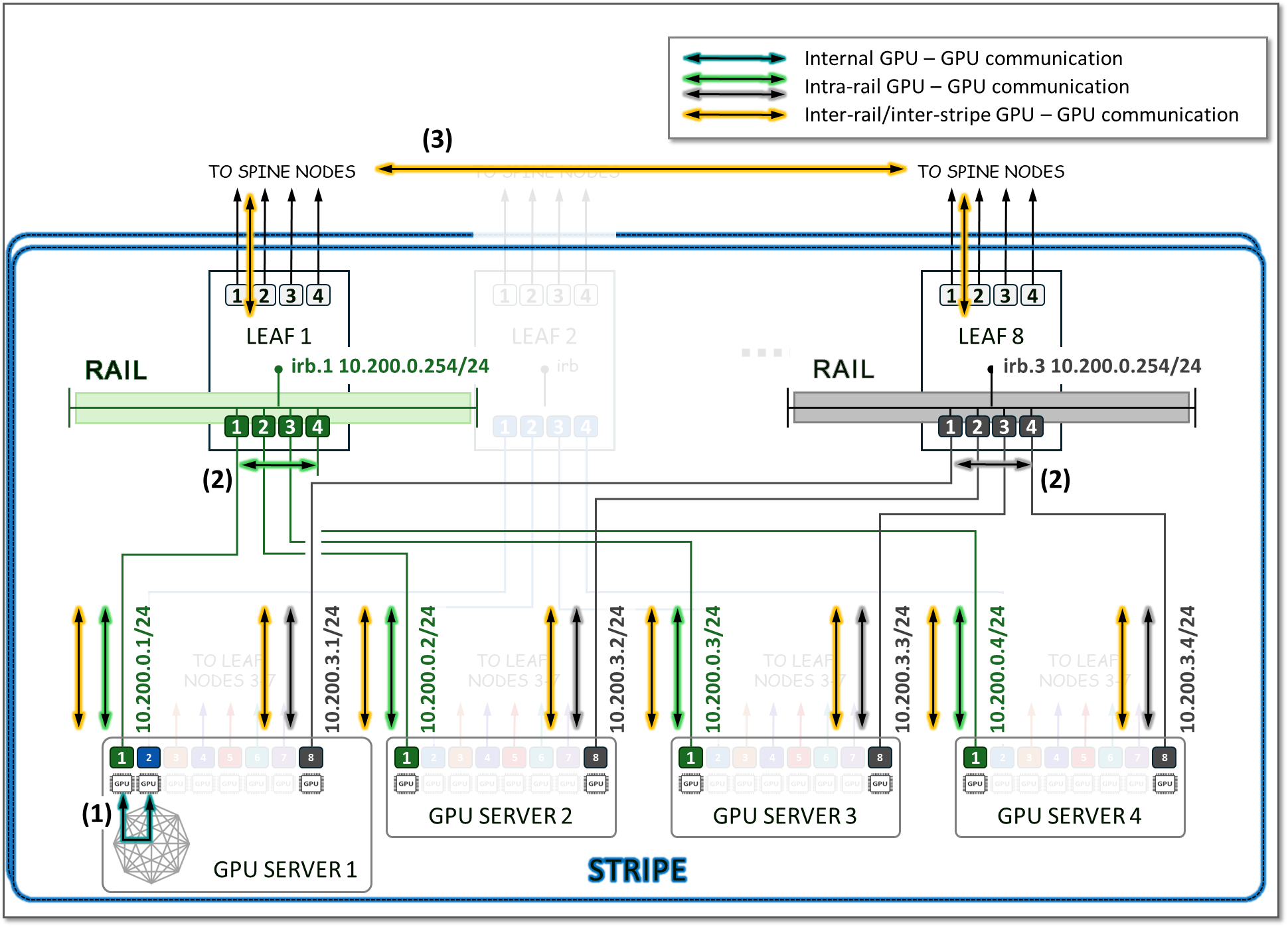
Traffic between GPUs on the same servers can be forwarded locally across the internal Server fabric (server architecture dependent). Traffic between GPUs in different servers happens across the GPU backend infrastructure, either within the same rail (intra-rail), or in different rails (inter-rail/inter-stripe).

Intra-rail traffic is processed at the local leaf node. Following this design, data between GPUs on different servers (but in the same stripe) is always moved on the same rail and across one single switch, while data between GPUs on different rails needs to be forwarded across the spines.

Using the example for calculating the number of servers per stripe provided in the previous section, we can see how:

• Communication between GPU 1 and GPU 2 in server 1 happens across the server’s internal fabric (1),
• Communication between GPU 1 in servers 1- 4, and between GPU 8 in servers 1- 4 happens across Leaf 1 and Leaf 8 respectively (2), and
• Communication between GPU 1 and GPU 8 (in servers 1- 4) happens across leaf1, the spine nodes, and leaf8 (3)

This is illustrated in Figure 15.

Figure 15: Inter-Rail vs. Intra-Rail GPU-GPU Communication

Most vendors implement local optimization to minimize latency for GPU-to-GPU traffic. Traffic between GPUs of the same number remains intra-rail. Figure 16 shows an example where GPU1 in Server 1 communicates with GPU1 in Server 2. The traffic is forwarded by Leaf Node 1 and remains within Rail 1.

Additionally, a NCCL feature known as PXN can be enabled to leverage internal fabric connectivity between GPUs within a server, where data is first moved to a GPU on the same rail as the destination, then send it to the destination without crossing rails. For example, if GPU4 in Server 1 wants to communicate with GPU5 in Server 2, and GPU5 in Server 1 is available across the internal fabric, the traffic naturally prefers this path to optimize performance and keep GPU-to-GPU communication intra-rail.

Figure 16: GPU to GPU Inter-Rail Communication Between Two Servers with PXN.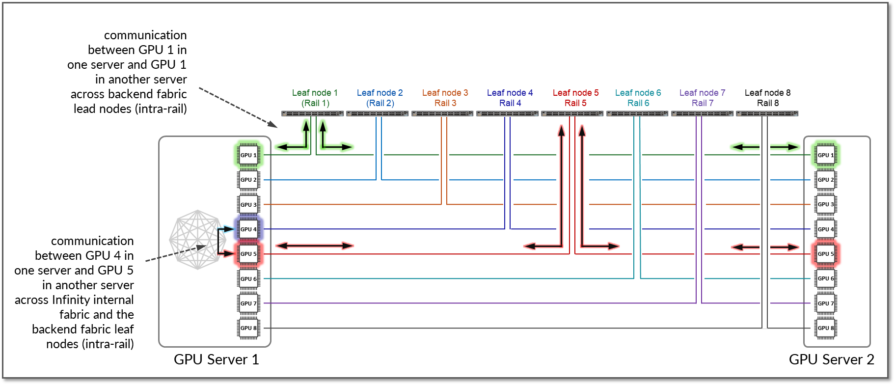

If this path is not feasible because of workload or service constraints, or because PXN is disabled the traffic will use RDMA (off-node NIC-based communication). In such case, GPU4 in Server 1 communicates with GPU5 in Server 2 by sending data directly over the NIC using RDMA, which is then forwarded across the fabric, as shown in Figure 17.

Figure 17: GPU to GPU Inter-Rail Communication Between Two Servers without PXN.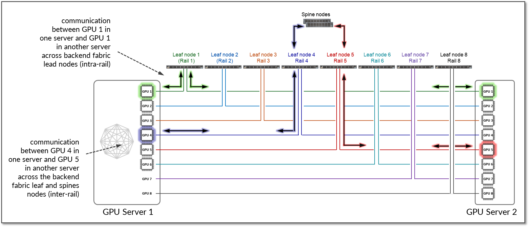

While PXN is a NCCL (NVIDIA Collective Communication Library) it is also supported by AMDs ROCm Communication Collectives Library. To enable or disable PXN use the variable NCCL_PXN_DISABLE

Rail Alignment and Local Optimization Considerations with GPU multitenancy

When implementing multitenancy in GPU fabrics, additional considerations apply regarding how GPUs are assigned and how communication between GPUs is handled.

Server Isolation model

In the server-isolation model, all GPUs in a server are dedicated to a single tenant. In this model, direct communication between GPUs within the same server is both appropriate and desirable. Placing the network interfaces connecting servers assigned to different tenants into different VRFs on the leaf nodes is sufficient to keep tenants separated across the network, but GPU-to-GPU communication also needs to be consider. Local optimization ensures that GPU-to-GPU communication follows the most optimal internal path:

• • GPUs within the same server communicate using the server’s internal mechanisms.
  • GPUs in different servers but connected to the same stripe can communicate across leaf nodes.
  • GPUs located in servers that connect to different stripes communicate through the spine layer, where traffic is encapsulated in VXLAN and routed across the EVPN/VXLAN fabric.

Note:

The examples in this section show possible paths for data between GPUs. The actual path depends on collectives (All-Gather, All-Reduce, All-To-All, etc) and topology algorithm (ring, tree, etc.) selected. Also, when a job runs there might be multiple topologies at the same time (e.g. multiple rings) following different path, built to increase efficiency. The actual path can be found in the slurm logs as shown in the example:

where:

X[Y] -> A[B]:

• X Source GPU global index.
• Y Local GPU index (within the node).
• A Destination GPU global index.
• B Local GPU index.

[send] / [receive]: Direction from the perspective of the process writing the log.

NET/IBext/N or NET/IBext/N(P):

• N=InfiniBand interface index (N)
• P (in parentheses) = NIC port or peer rank.

GDRDMA: GPUDirect RDMA, which means data goes directly between GPUs' memory over RDMA-capable NICs without CPU involvement. This is optimal for latency and bandwidth. Enables direct data exchange between the GPU and a third-party peer device using standard features of PCI Express. It is based on a kernel module called nv_peer_mem, which allows Mellanox and other RDMA-enabled NICs to directly read and write CUDA memory using NIC RDMA paths. NCCL provides routines optimized for high bandwidth and low latency over PCIe, NVLink, and NVIDIA Mellanox Network.

P2P/IPC: Point-to-Point (P2P) transport in the NVIDIA Collective Communications Library (NCCL). It enables GPUs to communicate directly with each other without going through the host CPU or network. NCCL provides inter-GPU communication primitives that are topology-aware and can be easily integrated into applications.

Example 1

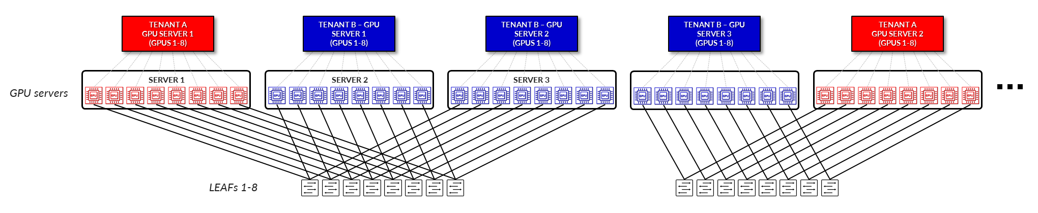
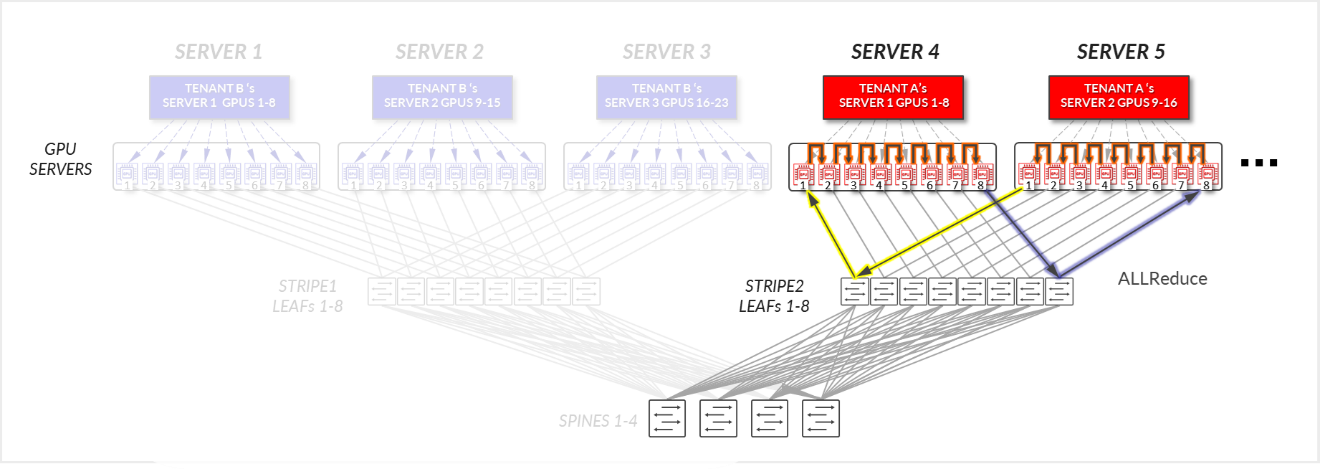
Consider the example depicted in Figure 18, where Tenant A has been assigned SERVERS 4 and SERVER 5, in the same stripe and Tenant B has been assigned SERVER 1, SERVER 2, and SERVER 3, also in the same stripe.

Figure 18: Server-isolation model GPU to GPU communication example 1

For Tenant A:

• GPUs 1-8 in SERVER 4, and GPUs 1-8 in SERVER 5 communicate internally within their respective servers, as explained in the section of Local Optimization.
• GPUs 1 and 8 in SERVER 4 communicate with GPUs 1 and 8 in SERVER 5 across the leaf and spine nodes - Intra-rail (traffic stays at the leaf node level).

Figure 19: Server-isolation model GPU to GPU communication example 1 – Tenant A

• • You can see how a ring logical topology is established interconnecting the 16 GPUs assigned to Tenant A, without any traffic crossing the Spine nodes.

Figure 20: Server-isolation model GPU to GPU communication example 1 – Tenant A Ring topology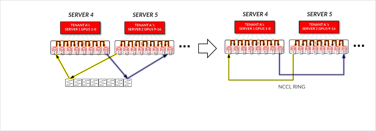

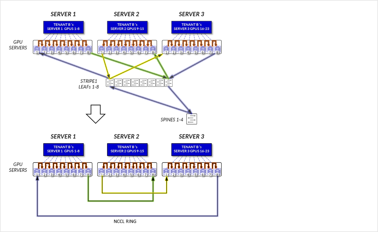
For Tenant B:

• GPUs 1-8 SERVER 1, GPUs 1-8 in SERVER 2, and GPUs 1-8 in SERVER3, communicate internally within their respective servers, as explained in the section of Local Optimization.
• GPUs 1 in SERVER 1 communicate GPUs 1 in SERVER 3 communicate with each other across the leaf nodes - Intra-rail (traffic stays at the leaf node level).
• GPUs 8 in SERVER 1 communicate GPUs 8 in SERVER 3 communicate with each other across the leaf nodes - Intra-rail (traffic stays at the leaf node level).
• GPUs 8 in SERVER 1 and GPUs 1 in SERVER 2 communicate across the leaf and spine nodes - Inter-rail. This is needed to complete the ring.

Figure 21: Server-isolation model GPU to GPU communication example 1 – Tenant B

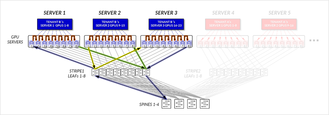
Figure 22: Server-isolation model GPU to GPU communication example 1 – Tenant B Ring topology

Example 2

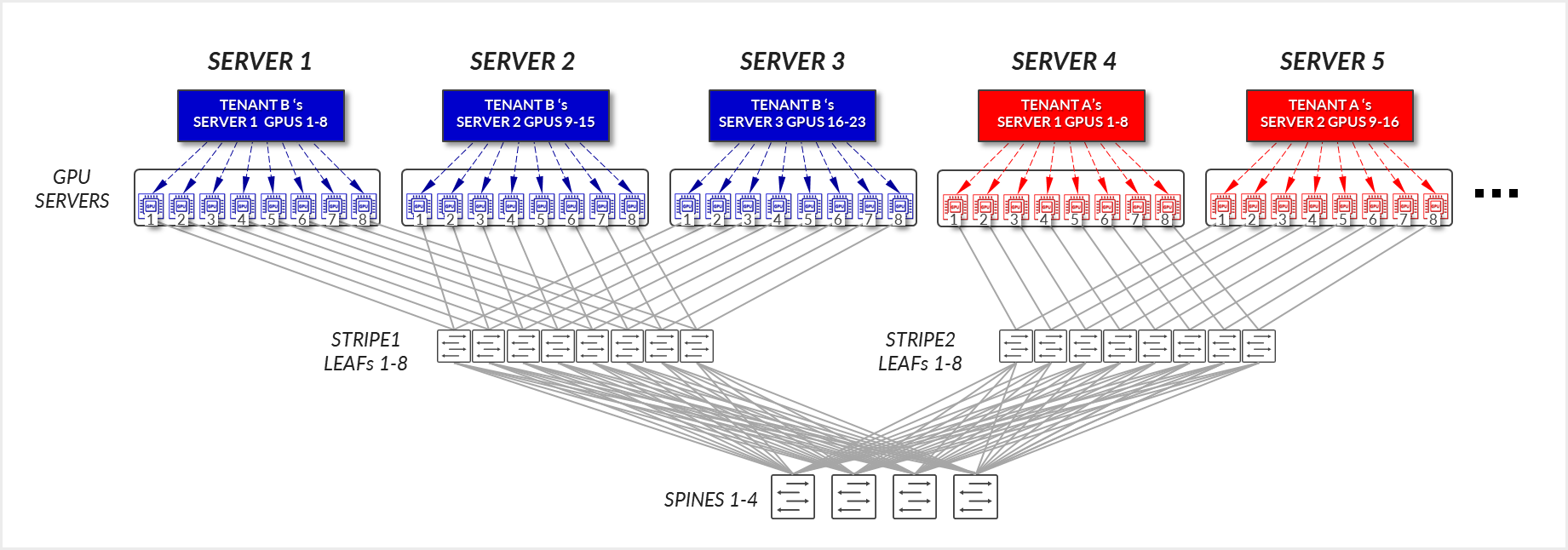
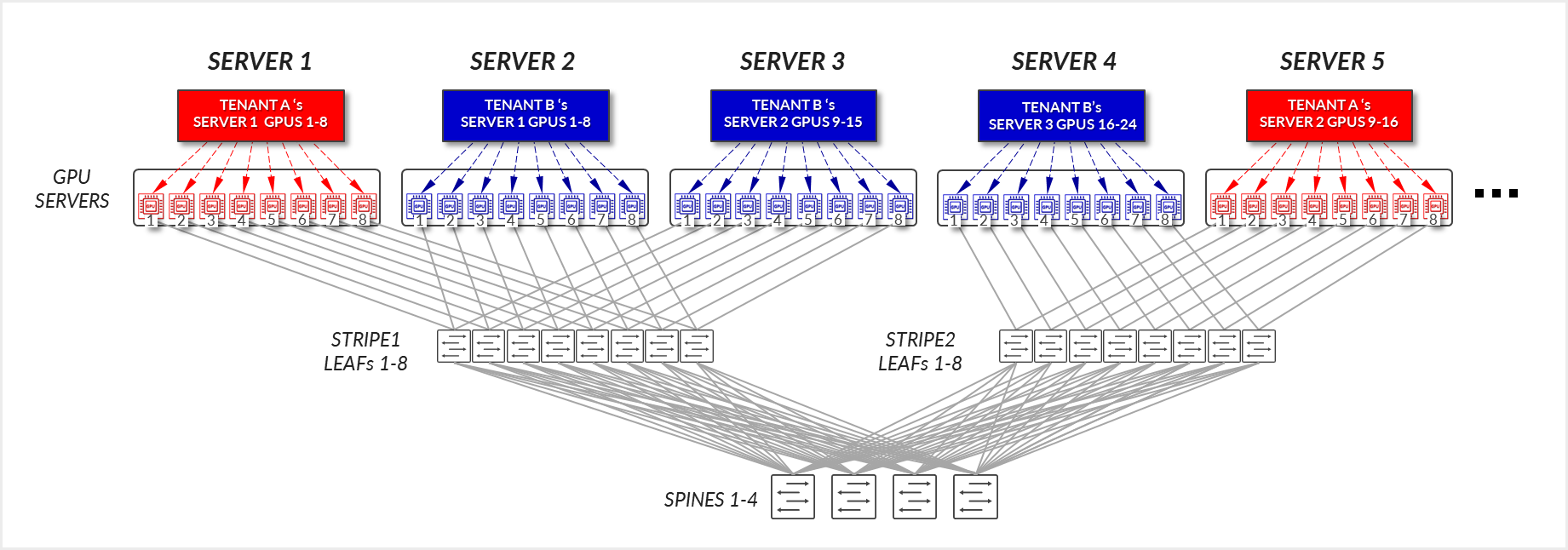
Now consider the example depicted in Figure 23, where Tenant A has been assigned Servers 1 and Server 5 in two different stripes, and Tenant B has been assigned Server 2, and Server 3, in the same stripe, and Server 4 in a different stripe.

Figure 23: Server-isolation model GPU to GPU communication example 2

For Tenant A:

• GPUs 1-8 in SERVER 1, and GPUs 1-8 in SERVER 5 communicate internally within their respective servers.
• GPUs 1 in SERVER 1 and GPUs 1 in SERVER 5 communicate across the leaf and spine nodes - Inter-stripe traffic.
• GPUs 8 in SERVER 1 and GPUs 8 in SERVER 5 communicate across the leaf and spine nodes - Inter-stripe traffic. This is needed to complete the ring.

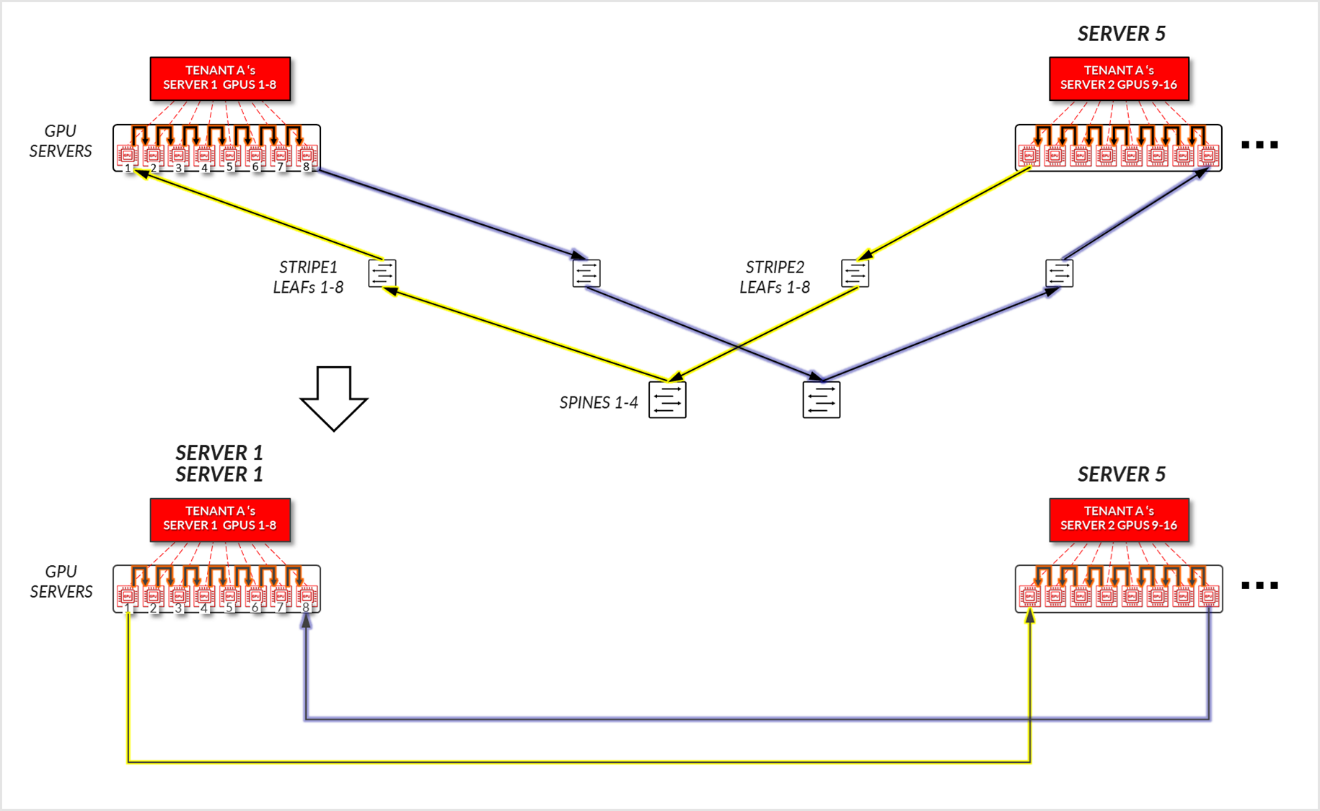
Figure 24: Server-isolation model GPU to GPU communication example 2 – Tenant A

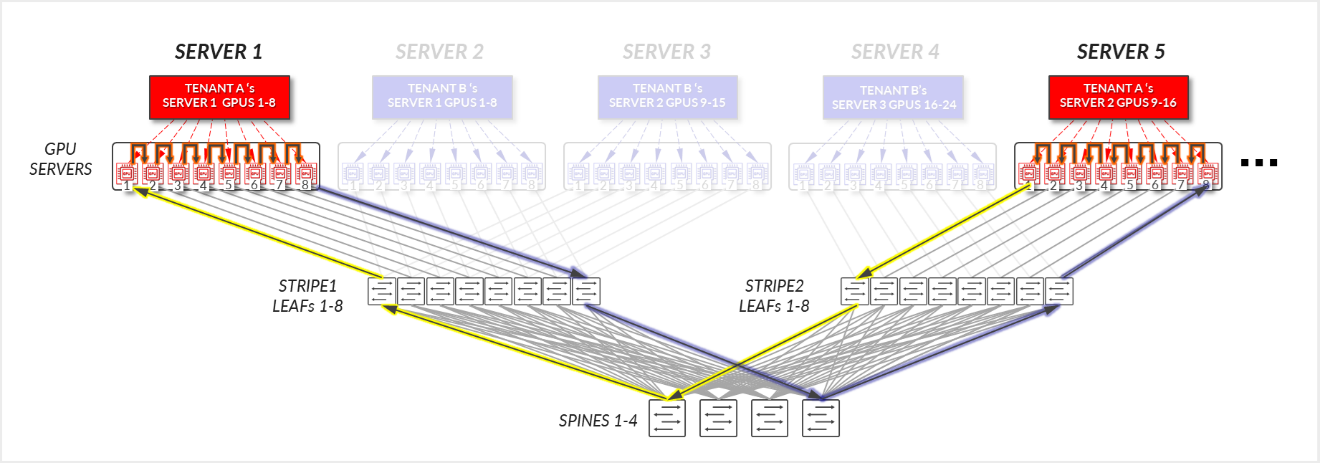
Figure 25: Server-isolation model GPU to GPU communication example 2 – Tenant A Ring topology

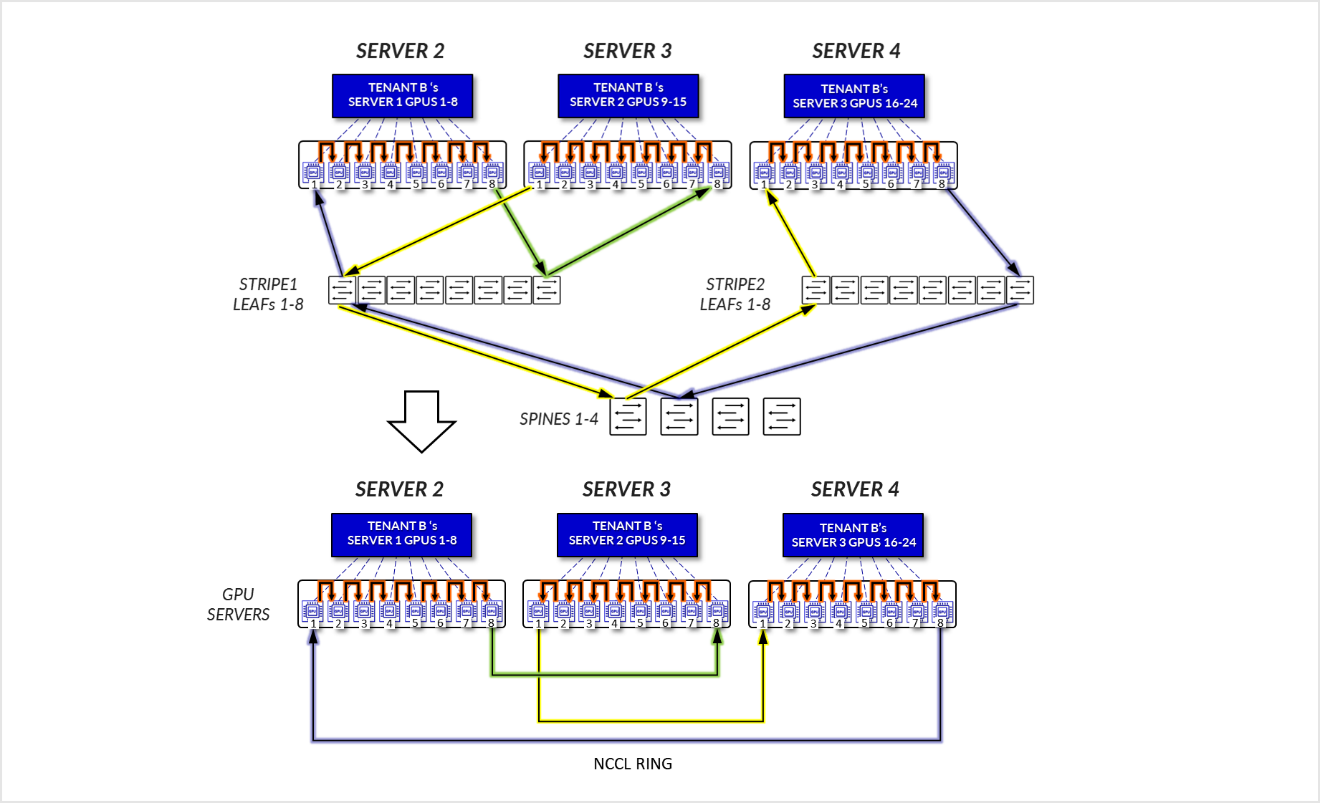
For Tenant B:

• GPUs 1-8 SERVER 2, GPUs 1-8 in SERVER 3, and GPUs 1-8 in SERVER4, communicate internally within their respective servers.
• GPUs 1 in SERVER 2 and GPUs 1 in SERVER 4 communicate across the leaf and spine nodes - Inter-stripe traffic.
• GPUs 8 in SERVER 4 and GPUs 8 in SERVER 3 communicate across the leaf and spine nodes - Inter-stripe traffic.
• GPUs 1 in SERVER 3 and GPUs 8 in SERVER 2 communicate across the leaf and spine nodes – Inter-rail. This is needed to complete the ring.

Figure 26: Server-isolation model GPU to GPU communication example 2 – Tenant B

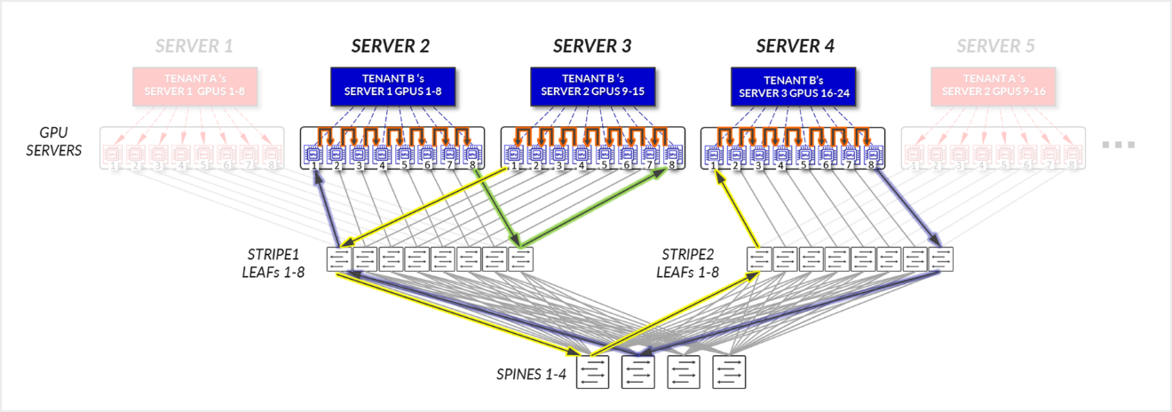
Figure 27: Server-isolation model GPU to GPU communication example 2 – Tenant B Ring topology

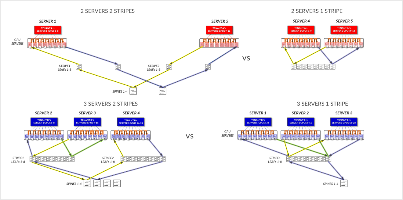
Comparing the data flow in Examples 1 and 2, shows how the assignment of the Servers to a tenant could influence the performance of the jobs.

Figure 28: Server-isolation with servers in same stripe vs servers in different stripes

GPU Isolation model

In the GPU-isolation model, different GPUs in the same server can be assigned to different tenants. Also, a tenant might be assigned GPUs in multiple servers across multiple stripes. As for the server isolation model, where the assigned GPUs are located will affect the path and potentially the performance.

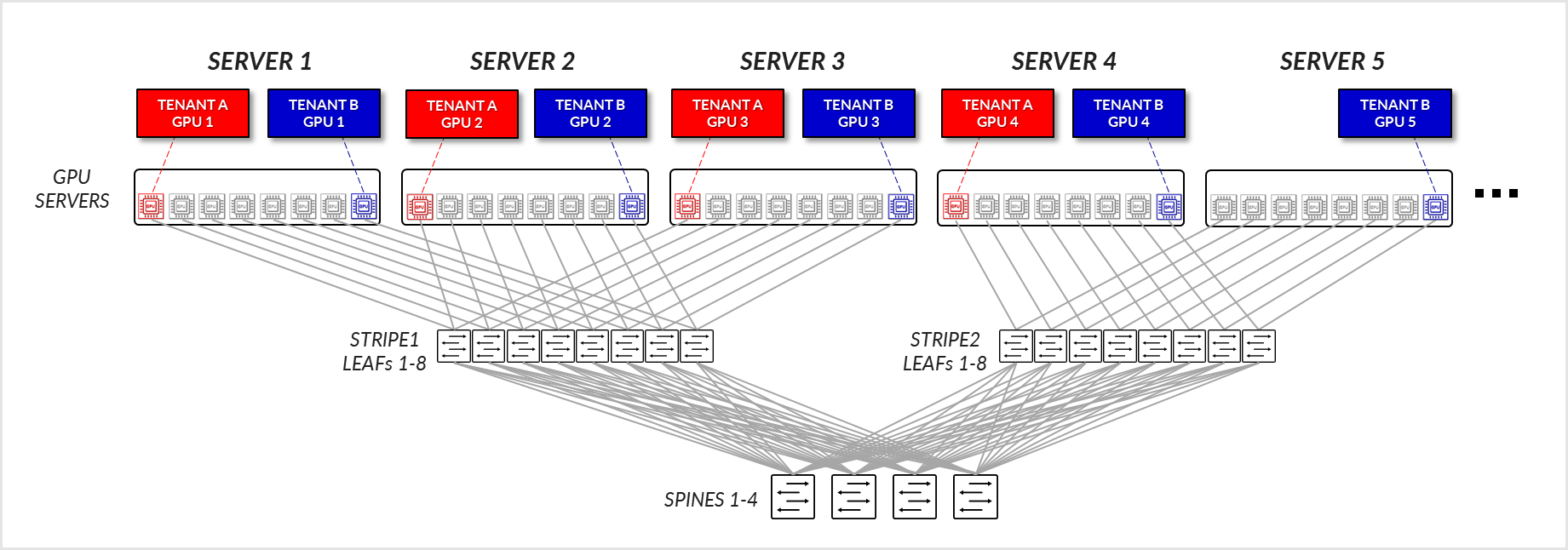
Example 1

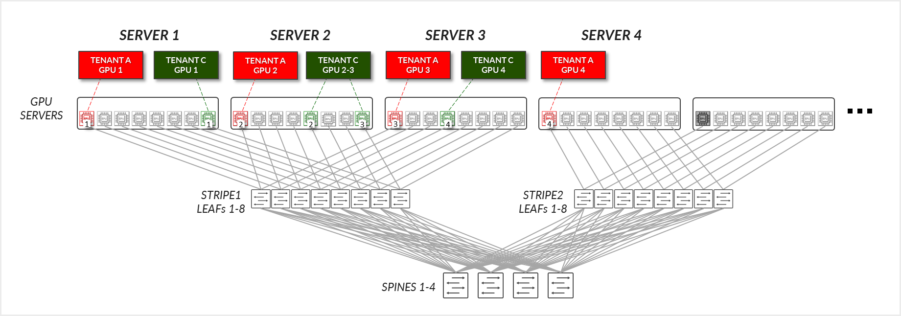
Consider the example depicted in Figure 29, where Tenant A has been assigned GPU1 on SERVERs 1-4, and Tenant B has been assigned GPU8 on SERVERs 1-5.

Figure 29: GPU-isolation model GPU to GPU communication example 1

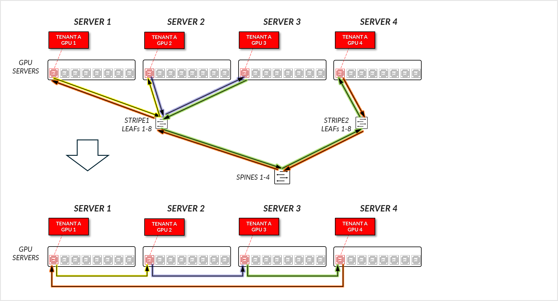
For Tenant A:

• Tenant A’s GPUs 1, 2, and 3 communicate with each other across the leaf node where they are connected. (Intra-rail)
• Tenant A’s GPUs 1, 2, and 3 communicate with GPU 4 communicate across the leaf and spine nodes.

Figure 30: GPU-isolation model GPU to GPU communication example 1 – Tenant A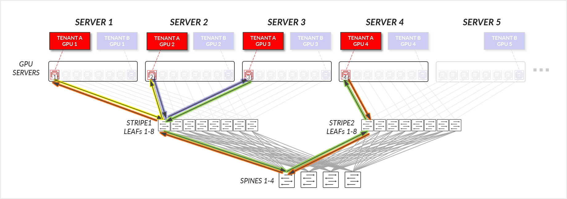

Figure 31: GPU-isolation model GPU to GPU communication example 1 – Tenant A ring topology

For Tenant B, a similar communication path is established.

Example 2

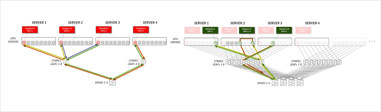
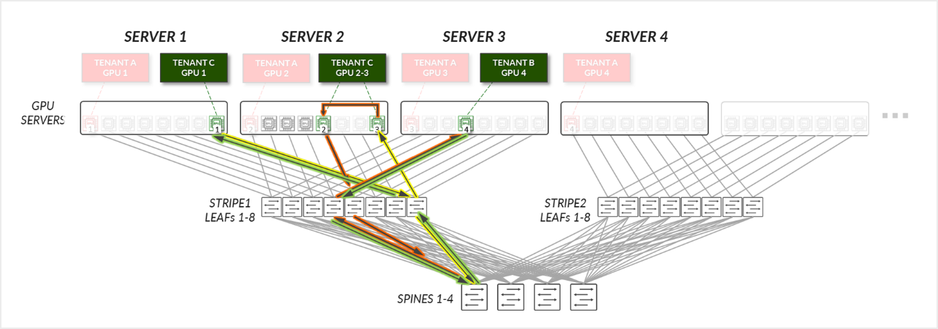
Now Consider the example depicted in Figure 32, where Tenant C has been assigned GPUs 8 on SERVER 1, GPUs 5 & 8 on SERVER 2, and GPU 4 on SERVER 3 (corresponding to Tenant C's GPUs 1-4 in the diagram).

Figure 32: GPU-isolation model GPU to GPU communication example 2

For Tenant C:

• Tenant C’s GPUs 2 and 3 (on the same server), communicate internally within their server.
• Tenant C's GPU 3 (SERVER 2) and GPU 4 (SERVER 3) communicate across the leaf and spine nodes.
• Tenant C's GPU 4 (SERVER 3) and GPU 1 (SERVER 1) communicate across the leaf and spine nodes.
• Tenant C's GPU 1 (SERVER 1) and GPU 2 (SERVER 2) communicate across the leaf and spine nodes.

Figure 33: GPU-isolation model GPU to GPU communication example 2 – Tenant C

When comparing examples 1 and 2, it becomes clear how rail alignment and proper server or GPU assignment strategies are critical to achieving optimal GPU-to-GPU communication efficiency on a scale.

Tenant A in Example 1, has been assigned GPU0 on Servers 1-4, thus communication mostly stays at the leaf level. Tenant C in Example 2 has been assigned GPUs 8 on SERVER 1, GPUs 5 & 8 on SERVER 2, and GPU 4 on SERVER 3, so communication must go across the spines, introduces additional latency and potential congestion Both Tenant A and Tenant C have been assigned the same number of GPUs, but communication between their GPUs follows different paths, which could result in varying performance levels.

Figure 34: GPU-isolation with servers in same stripe vs servers in different stripes