Managing Congestion Using RED Drop Profiles and Packet Loss Priorities

The second parameter defines the drop probabilities across the range of delay-buffer occupancy, supporting the random early detection (RED) process. When the number of packets queued is greater than the ability of the router or switch to empty a queue, the queue requires a method for determining which packets to drop from the network. To address this, the Junos OS provides the option of enabling RED on individual queues.

Depending on the drop probabilities, RED might drop many packets long before the buffer becomes full, or it might drop only a few packets even if the buffer is almost full.

A drop profile is a mechanism of RED that defines parameters that allow packets to be dropped from the network. Drop profiles define the meanings of the packet loss priorities.

When you configure drop profiles, there are two important values: the queue fullness and the drop probability. The queue fullness represents a percentage of the memory used to store packets in relation to the total amount that has been allocated for that specific queue. Similarly, the drop probability is a percentage value that correlates to the likelihood that an individual packet is dropped from the network. 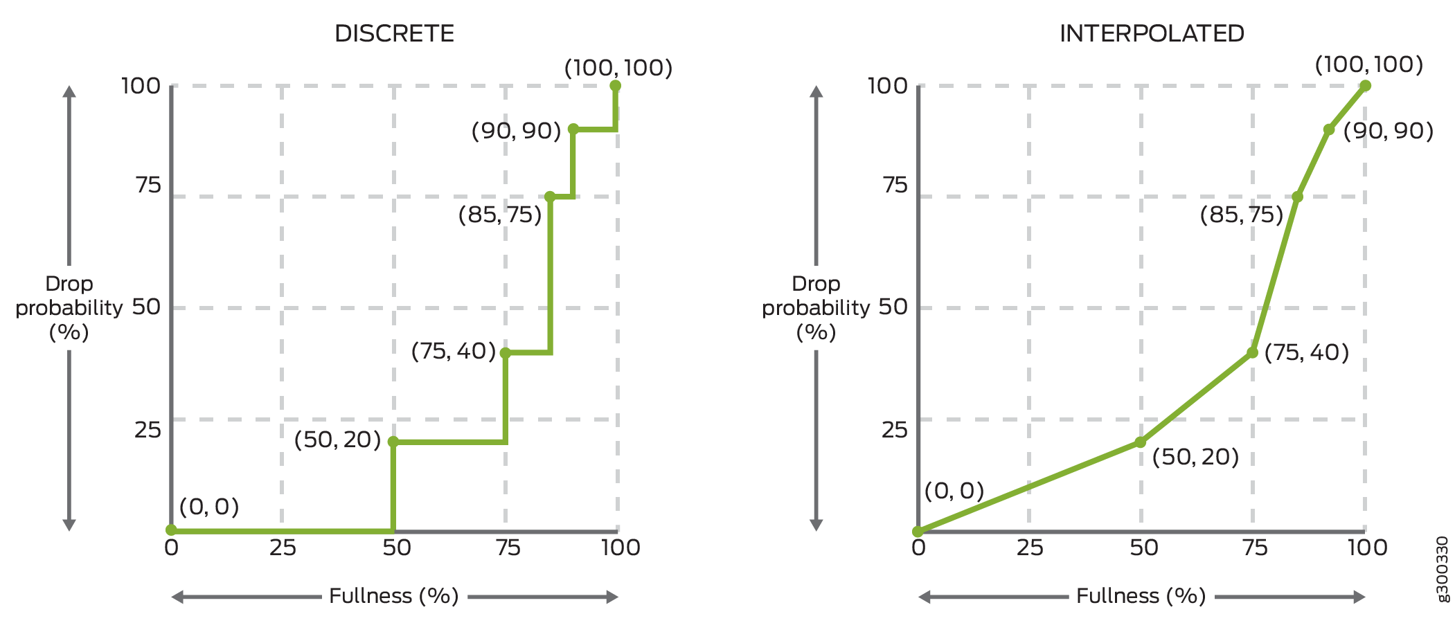How these two variables function is illustrated in graph format, as shown in Figure 1.

The maximum number of queue fullness levels supported per drop profile is based on the line card:

• Physical or logical interfaces hosted on MICs in Queuing or Enhanced Queuing MPCs for MX Series routers support up to 64 (fill level, drop probability) pairs per discrete or interpolated drop profile.

• Physical or logical interfaces hosted on Enhanced Queuing DPCs for MX Series routers support up to 64 (fill level, drop probability) pairs per discrete drop profile or 2 pairs per interpolated drop profile. For more information, see Configuring WRED on Enhanced Queuing DPCs.

• Physical or logical interfaces hosted on IQ2 PICs or IQE PICs support up to two (fill level, drop probability) pairs per discrete or interpolated drop profile.

• PTX Series routers running Junos OS and PTX10003 routers running Junos OS Evolved support up to 64 (fill level, drop probability) pairs per discrete or interpolated drop profile.

• Other PTX Series routers running Junos OS Evolved support up to two (fill level, drop probability) pairs per interpolated drop profile. A single-pair drop profile is discrete. Two pairs will be interpolated.

Figure 1 shows both a discrete and an interpolated graph. Although the formation of these graph lines is different, the application of the profile is the same. When a packet joins the tail of the queue, a random number between 0 and 100 is calculated by the router or switch. This random number is plotted against the drop profile using the current queue fullness of that particular queue. When the random number falls above the graph line, the packet is transmitted onto the physical media. When the number falls below the graph line, the packet is dropped from the network.

Figure 1: Discrete and Interpolated Drop Profiles

Drop profiles are created by defining multiple fill levels and drop probabilities and can be illustrated by graphs in which the x axis represents the fill level and the y axis represents the drop probability.

To create the discrete profile graph as shown in Figure 1 on the left, the software begins at the bottom-left corner, representing a 0-percent fill level and a 0-percent drop probability. This configuration creates a line horizontally to the right on the fullness level (l) x-axis until it reaches the first defined fill level, 50-percent for this configuration, which is designated to have a drop probability (p) of 20-percent. The software then continues the line horizontally along the fill level until the next drop probability is reached at the designated data point of 75-percent fill level, which has a designated drop-probability of 40-percent. The line is then continued horizontally to the next fill level of 85-percent and the designated drop probability of 75-percent. The line continues horizontally to the next designated fill level of 90-percent, which has a designated drop probability of 90-percent, and a line is created to data point 90-percent (l), 90-percent (p) (l90 p90). From the l90 p90 point, the line continues horizontally to the 100-percent fill level, which has a drop probability of 100 percent, at which the line rises to the end-point of 100-100, which is 100 percent fill level with a 100 percent drop probability.

If an interpolated drop profile is specified, in the first quadrant the initial line segment spans from the origin (0,0) to the next defined point. From that defined fill-level/drop-probability point, a second line runs to the next point, and so forth, until a final line segment connects (100, 100). The software automatically constructs a drop profile containing 64 fill levels at drop probabilities that approximate the calculated line segments.

You can create a smoother graph line by configuring the profile with the interpolate statement. This enables the software to automatically generate 64 data points on the graph beginning at (0, 0) and ending at (100, 100). Along the way, the graph line intersects specific data points that you have defined.

Loss priorities allow you to set the priority of dropping a packet. Loss priority affects the scheduling of a packet without affecting the packet’s relative ordering. You can use the packet loss priority (PLP) bit as part of a congestion control strategy. You can use the loss priority setting to identify packets that have experienced congestion. Typically you mark packets exceeding some service level with a high loss priority. You set loss priority by configuring a classifier or a policer. The loss priority is used later in the workflow to select one of the drop profiles used by RED.

You specify drop probabilities in the drop profile section of the class-of-service (CoS) configuration hierarchy and map them to corresponding loss priorities in each scheduler configuration. For each scheduler, you can configure multiple separate drop profiles, one for each combination of loss priority (low, medium-low, medium-high, or high)l.

You can configure a maximum of 32 different drop profiles.

To configure RED drop profiles, include the following statements at the [edit class-of-service] hierarchy level:

If you configure no drop profiles on Juniper Networks M320 Multiservice Edge Routers or T Series Core Routers, random early detection (RED) is in effect by default and functions as the primary mechanism for managing congestion. In the default RED drop profile, when the fill-level is 0 percent, the drop probability is 0 percent. When the fill-level is 100 percent, the drop probability is 100 percent.

As a backup method for managing congestion, tail dropping takes effect when congestion of small packets occurs. On M320 and T Series Core Routers, the software supports tail-RED, which means that when tail dropping occurs, the software uses RED to execute intelligent tail drops. On other routers, the software executes tail drops unconditionally.