Querying the Metrics Database
Introduction
The metrics database uses the TimescaleDB extension to efficiently manage time series data from Paragon Active Assurance, providing additional functions for data aggregation and rollup.
In this chapter we will describe the database objects and fields of the metrics database and their usage within an SQL query.
For full coverage of TimescaleDB features, go to docs.timescale.com.
Database Objects to Query
Each plugin in Paragon Active Assurance has a number of database views which the user can query:
- one view for tests
- five views for monitors with metrics aggregated at different granularities: 10 seconds (raw), 1 minute, 5 minutes, 30 minutes, and 60 minutes.
The naming convention for the view objects is the following:
-
vw_(monitor|test)_metrics_<plugin_name>for raw metrics data -
vw_monitor_metrics_minute<minutes>_<plugin_name>for metrics aggregated over time intervals of size<minutes>for the purpose of monitoring.
For example, the HTTP plugin has the following database objects that can be queried:
vw_test_metrics_http
vw_monitor_metrics_http
vw_monitor_metrics_minute1_http
vw_monitor_metrics_minute5_http
vw_monitor_metrics_minute30_http
vw_monitor_metrics_minute60_http
Each view contains two categories of information:
-
measurement: This is metadata such as the name of the test or monitor and the Test Agent(s) used. It is needed to retrieve the information related to a task in a test or monitor, and it should be included in the WHERE clause of an SQL statement to narrow down the search. Examples of fields in this category are:
- Common to monitoring and testing:
account_short_name,task_name,stream_name,plugin_name - Specific to testing:
test_name,test_step_name,periodic_test_name - Specific to monitoring:
monitor_name,task_started,monitor_tags
monitor_name, task_name, stream_name, test_name, test_agent_name
- Common to monitoring and testing:
- metric: This is data collected in the network at a given point in time, such as throughput, delay, and jitter.
The _time column is common to all views and must be included in each
query. However, the set of metrics returned depends on the task type: for example, an HTTP
measurement will have a different set of metrics from a Ping measurement.
The columns holding specific measurements differ from one task to another, and they are usually part of the metrics table in the view definition.
For example, the vw_monitor_metrics_http view contains:
connect_time_avg,
first_byte_time_avg,
response_time_min,
response_time_avg,
response_time_max,
size_avg,
speed_avg,
es_timeout,
es_response,
es
Running Queries in TimescaleDB
To run queries in TimescaleDB it is important to:
- identify the measurement task that collects the metrics
- identify and set the time interval of interest
- set the data granularity for the metrics.
- Identifying the Task of Interest
- Setting the Time Interval of Interest
- Setting Data Granularity for Metrics
Identifying the Task of Interest
Metrics collected during execution of a test or monitor are produced by all the measurement tasks defined in the test or monitor. To uniquely identify such a task in the metrics database, it is essential to retrieve the right information from Control Center.
Identifying a Monitor Task
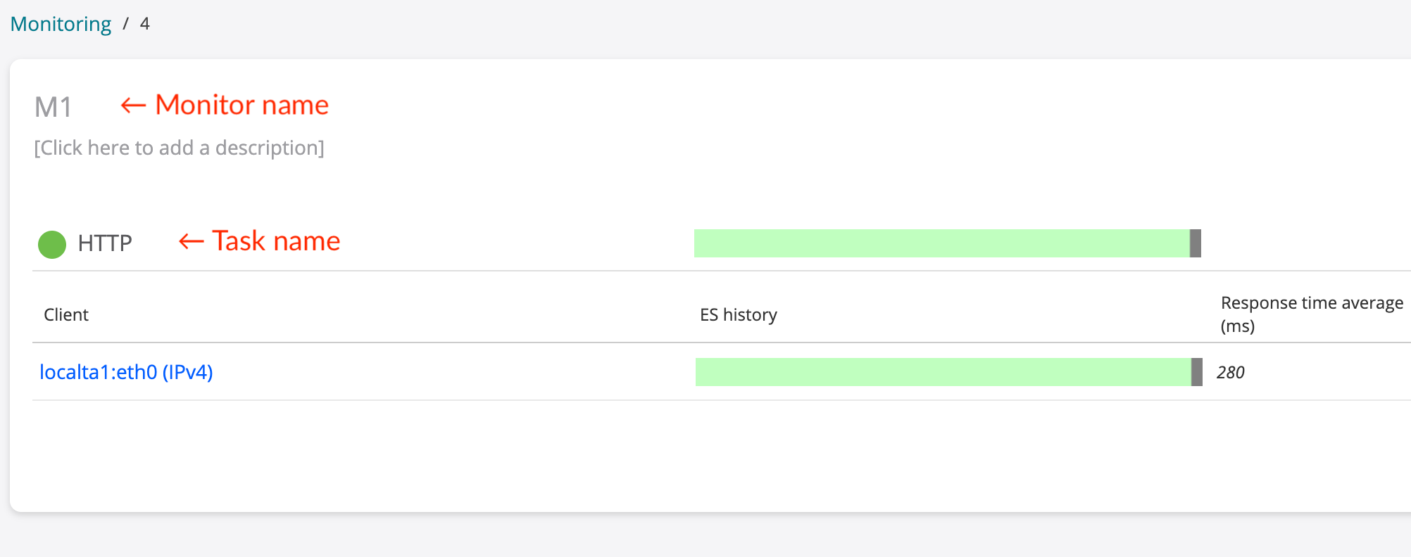
- In Control Center, click the Monitoring button on the left-side bar.
- Click List.
-
Click the monitor name in the list and note the name of the task of interest. An example is shown below:
-
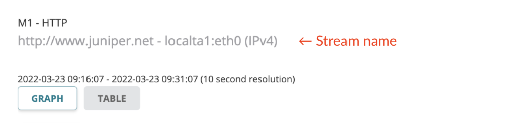
Click the client name and note the name of the stream, which is displayed as shown in the following image:
-
Run this query, where
monitor_name,task_name, andstream_nameare taken from the Control Center GUI as just shown:SELECT DISTINCT monitor_id,monitor_name, task_id,task_name, id as stream_id,stream_name FROM streams WHERE monitor_name = '<monitor_name>' AND task_name = '<task_name>' AND stream_name = '<stream_name>';Take note of
monitor_id,task_idandstream_idin the output. For example:-[ RECORD 1 ]+---------------------------------------------- monitor_id | 6 monitor_name | M1 task_id | 8 task_name | HTTP stream_id | 10 stream_name | http://www.juniper.net - localta1:eth0 (IPv4)
Identifying a Test Task
This is similar to monitor task identification (see above) except that in the Control Center GUI, you click the Tests button on the left-side bar. The query is also modified accordingly:
SELECT DISTINCT test_id,test_name,
                task_id,task_name,
                id as stream_id,stream_name
FROM streams
WHERE test_name = '<test_name>'
AND task_name = '<task_name>'
AND stream_name='<stream_name>';
Setting the Time Interval of Interest
To ensure that we are querying data in the right time interval, it is important to know the time zone of reference in the metrics database and whether it differs from the time representation in Control Center.
To get the current time zone of the database, run this query:
SELECT now(),current_setting('TIMEZONE');Example of output:
              now              | current_setting
-------------------------------+-----------------
 2022-03-22 18:06:01.247507+00 | Etc/UTC
(1 row)
In this case, the current time zone of the database is UTC, so all time intervals are represented in UTC.
To convert a local time zone to UTC, perform the following steps:
- Define the local time in the format
YYYY-MM-dd HH:mm(<local_time>). -
Select the appropriate local time zone:
-
Run this query (
<continent>is the name of the continent):SELECT name FROM pg_timezone_names WHERE name ilike '<continent>/%' ORDER BY name;
Select the time zone name corresponding to the city closest to you and assign it to
.local_time_zone(for example,America/New_York)
-
-
Run the query below to get the time in UTC:
SELECT TIMESTAMP '<local_time>' AT TIME ZONE '<local_time_zone>';
Example
Here is how to convert the time 2021-12-16 15:00 from Pacific Time to UTC:
-
<local_time>is2021-12-16 15:00. -
Run this query to retrieve time zones in the Americas:
SELECT name
FROM pg_timezone_names
WHERE name ilike 'America/%'
ORDER BY name;
- Select
America/Los_Angelesfrom the list. -
Run this query to have the time zone converted:
SELECT TIMESTAMP '2021-12-16 15:00' AT TIME ZONE 'America/Los_Angeles';
        timezone
------------------------
 2021-12-16 23:00:00+00
(1 row)
Setting Data Granularity for Metrics
Depending on the time interval of interest, it is possible to run queries on metrics using either
- the predefined views available in TimescaleDB directly, or
- the predefined views as a data source for metrics aggregation on custom time intervals.
Below is an example. Suppose we are analyzing the stream below:
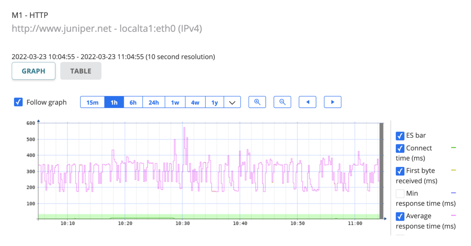
Here we have:
-
monitor_id=6for theM1monitor -
task_id=8for theHTTPtask inM1 -
stream_id=10for the stream namedhttp://www.juniper.net - localta1:eth0 (IPv4) - Time interval delimited by
<time_start>and<time_end>:-
<time_start>=2022-03-23 10:04:55+00 -
<time_end>=2022-03-23 11:04:55+00
-
Queries on Predefined Views
These queries are recommended if the data granularity of interest is already present in TimescaleDB.
The format of the query is:
SELECT
  -- time field
  _time AS "time",
  -- metric
  response_time_avg as "avg_response_time"
FROM
  -- data source
  <data_source>
WHERE
  -- time interval to analyze
  _time between '<time_start>' AND '<time_end>'
  AND
  -- constraints on metadata
  monitor_id = <monitor_id>
  AND task_id = <task_id>
  AND _stream_id = <stream_id>;
The value of <data_source> is one of the objects listed in the
Database Objects to Query
section.
Example
Given the context described in the previous paragraphs, the query
SELECT
  -- time field
  _time AS "time",
  -- metric
  response_time_avg as "avg_response_time"
FROM
  -- data source
  vw_monitor_metrics_minute5_http
WHERE
  -- time interval to analyze
  _time between '2022-03-23 10:04:55+00' AND '2022-03-23 11:04:55+00'
  AND
  -- constraints on metadata
  monitor_id = 6
  AND task_id = 8
  AND _stream_id = 10;
returns the value of the response_time_avg metric for a 5-minute
interval detected between 2022-03-23 10:04:55+00 and 2022-03-23
11:04:55+00 for the stream http://www.juniper.net - localta1:eth0
(IPv4) related to the task HTTP defined in the monitor
M1.
Below is an example of output that may be returned in this case:
          time          | avg_response_time
------------------------+--------------------
 2022-03-23 10:05:00+00 | 276.53887939453125
 2022-03-23 10:10:00+00 |  281.2976379394531
 2022-03-23 10:15:00+00 |  324.9761657714844
 2022-03-23 10:20:00+00 |  331.6311340332031
 2022-03-23 10:25:00+00 |  289.0729064941406
 2022-03-23 10:30:00+00 |  320.9573974609375
 2022-03-23 10:35:00+00 | 239.66653442382812
 2022-03-23 10:40:00+00 | 305.64556884765625
 2022-03-23 10:45:00+00 |  314.2927551269531
 2022-03-23 10:50:00+00 |  261.7337646484375
 2022-03-23 10:55:00+00 | 278.86273193359375
 2022-03-23 11:00:00+00 |  302.1415100097656
Queries with Custom Time Interval
To run aggregate functions on metrics based on time intervals, TimescaleDB introduced the concept of time buckets to customize the granularity of the measurements given an underlying data set.
The function time_bucket accepts arbitrary time intervals as well as
optional offsets and returns the bucket start time.
A user can apply aggregate functions on metrics grouped by the output from
time_bucket to define metrics granularity dynamically, if the time
interval of interest is not available in the TimescaleDB database.
The format of the query is:
SELECT
  -- time field
  time_bucket('<bucket_interval>',_time) as "time",
  -- metrics
  <metrics>
FROM
  -- data source
  <data_source>
WHERE
  -- time interval to analyze
  _time between '<time_start>' AND '<time_end>'
  AND
  -- constraints on metadata
  monitor_id = <monitor_id>
  AND task_id = <task_id>
  AND _stream_id = <stream_id>
GROUP BY time_bucket('<bucket_interval>',_time)
ORDER BY "time";
where <data_source> is one of the objects listed in the Database Objects to Query section
and <metrics> is a comma-separated list of metrics or an expression
involving metrics.
Metrics for HTTP tasks are likewise listed in the Database Objects to Query section.
<bucket_interval> denotes the interval width in use for rolling up
the metric values. A value for <bucket_interval> consists of a
number followed by a time unit such as:
-
s(orsecond) for seconds -
m(orminute) for minutes -
h(orhour) for hours -
d(orday) for days
Example
Given the context described in the previous paragraphs and the change
-
<bucket_interval>=10m(10-minute data granularity)
the query
SELECT
  -- time field
  time_bucket('10m',_time) as "time",
  -- metric
  percentile_cont(0.5) WITHIN GROUP (ORDER BY response_time_avg) as "avg_response_time"
FROM
  -- data source
  vw_monitor_metrics_http
WHERE
  -- time interval to analyze
  _time between '2022-03-23 10:04:55+00' AND '2022-03-23 11:04:55+00'
  AND
  -- constraints on metadata
  monitor_id = 6
  AND task_id = 8
  AND _stream_id = 10im
GROUP BY time_bucket('10m',_time)
ORDER BY "time";
returns the continuous 50% percentile value of the response_time_avg
metric within 10-minute intervals detected between 2022-03-23 10:04:55+00
and 2022-03-23 11:04:55+00 for the stream http://www.juniper.net
- localta1:eth0 (IPv4) related to the task HTTP defined in the
monitor M1.
The output returned in this case looks like this:
          time          | avg_response_time
------------------------+--------------------
 2022-03-23 10:00:00+00 | 288.12400817871094
 2022-03-23 10:10:00+00 |    338.41650390625
 2022-03-23 10:20:00+00 | 345.27549743652344
 2022-03-23 10:30:00+00 | 295.31700134277344
 2022-03-23 10:40:00+00 |  338.8695068359375
 2022-03-23 10:50:00+00 | 280.78651428222656
 2022-03-23 11:00:00+00 | 337.31800842285156
For better query performance, it is recommended that you use as data source the view with the coarsest granularity that guarantees acceptable data accuracy.