ACX7332 Network Cable and Transceiver Planning
Determining Transceiver Support for ACX7332
You can use the Hardware Compatibility Tool to find information about the pluggable transceivers and connector types supported by your Juniper Networks device. The tool also documents the optical and cable characteristics, where applicable, for each transceiver. You can search for transceivers by product—and the tool displays all the transceivers supported on that device—or by category, interface speed, or type. You can find the list of supported transceivers for the ACX7332 at https://apps.juniper.net/hct/product/.
If you face a problem running a Juniper Networks device that uses a third party optic or cable, the Juniper Networks Technical Assistance Center (JTAC) can help you diagnose the source of the problem. Your JTAC engineer might recommend that you check the third party optic or cable and potentially replace it with an equivalent Juniper Networks optic or cable that is qualified for the device.
|
FPC |
Transceiver Type |
Power Requirement |
Supported Operating Temperature |
|---|---|---|---|
|
ACX7K3‑FPC‑2CD4C (2 QSFP56-DD ports + 4 QSFP28 ports) |
QSFP56‑DD 400G (ZR+) |
23W (2xQSFP56‑DD 400G‑ZR+) |
40 ℃ at 6000 ft (standalone install) |
|
QSFP56‑DD 400G (ZR) |
20W (2xQSFP56‑DD 400G‑ZR) |
40 ℃ at 6000 ft (standalone install) |
|
|
QSFP56‑DD 400G |
14W (2xQSFP56-DD 400G) |
40 ℃ at 6000 ft (standalone install) |
|
|
QSFP28‑DD 200G and QSFP28 100G |
12.5W 2xQSFP28-DD 200G (7W) + 4xQSFP28 100G (5.5W) |
40 ℃ at 6000 ft (standalone install) 55 ℃ at 6000 ft (standalone install) 55 ℃ at 6000 ft (street cabinet-IP 65/IP 66 only) |
|
|
ACX7K3-FPC-16Y (16 SFP56 ports) |
SFP56 50G |
3W |
40 ℃ at 6000 ft (standalone install) |
|
2W |
40 ℃ at 6000 ft (standalone install) 55 ℃ at 6000 ft (standalone install) 55 ℃ at 6000 ft (street cabinet-IP 65/IP 66 only) |
||
|
SFP28 25G |
1.5W |
40 ℃ at 6000 ft (standalone install) 55 ℃ at 6000 ft (standalone install) 55 ℃ at 6000 ft (street cabinet-IP 65/IP 66 only) |
|
|
Fixed FPC (32 SFP28 ports + 8 QSFP28 ports) |
QSFP28 100G |
5.5W |
40 ℃ at 6000 ft (standalone install) 55 ℃ at 6000 ft (standalone install) 55 ℃ at 6000 ft (street cabinet-IP 65/IP 66 only) |
|
SFP28 25G |
1.5W |
40 ℃ at 6000 ft (standalone install) 55 ℃ at 6000 ft (standalone install) 55 ℃ at 6000 ft (street cabinet-IP 65/IP 66 only) |
Cable and Connector Specifications for ACX7332
The transceivers that an ACX7332 device supports use fiber-optic cables and connectors. The type of connector and the type of fiber depend on the transceiver type.
You can determine the supported cables and connectors for your specific transceiver by using the Hardware Compatibility Tool.
To maintain agency approvals, you must use only a properly constructed, shielded cable.
The terms multifiber push-on (MPO) and multifiber termination push-on (MTP) describe the same connector type. The rest of this topic uses MPO to mean MPO or MTP.
- 12-Fiber MPO Connectors
- 24-Fiber MPO Connectors
- 16-Fiber MPO Connectors
- CS Connector
- LC Duplex Connectors
12-Fiber MPO Connectors
The 12-fiber MPO connectors on Juniper Networks devices use two types of cables—patch cables with MPO connectors on both ends, and breakout cables with an MPO connector on one end and four LC duplex connectors on the other end. Depending on the application, the cables might use single-mode fiber (SMF) or multimode fiber (MMF). Juniper Networks sells cables that meet the supported transceiver requirements, but you are not required to purchase cables from Juniper Networks.
Ensure that you order cables with the correct polarity. Vendors refer to these crossover cables as key up to key up, latch up to latch up, Type B, or Method B. If you are using patch panels between two transceivers, ensure that the proper polarity is maintained through the cable plant.
Also, ensure that the fiber end in the connector is finished correctly. Physical contact (PC) refers to fiber that has been polished flat. Angled physical contact (APC) refers to fiber that has been polished at an angle. Ultra physical contact (UPC) refers to fiber that has been polished flat to a finer finish. You can determine the required fiber end with the connector type in the Hardware Compatibility Tool.
- 12-Fiber Ribbon Patch Cables with MPO Connectors
- 12-Fiber Ribbon Breakout Cables with MPO-to-LC Duplex Connectors
- 12-Ribbon Patch and Breakout Cables Available from Juniper Networks
12-Fiber Ribbon Patch Cables with MPO Connectors
You can use 12-fiber ribbon patch cables with socket MPO connectors to connect two transceivers of the same type—for example, 40GBASE-SR4-to-40GBASESR4 or 100GBASE-SR4-to-100GBASE-SR4. You can also connect 4x10GBASE-LR or 4x10GBASE-SR transceivers by using patch cables—for example, 4x10GBASE-LR-to-4x10GBASE-LR or 4x10GBASE-SR-to-4x10GBASE-SR—instead of breaking the signal out into four separate signals.
Table 2 describes the signals on each fiber. Table 3 shows the pin-to-pin connections for proper polarity.
|
Fiber |
Signal |
|---|---|
|
1 |
Tx0 (Transmit) |
|
2 |
Tx1 (Transmit) |
|
3 |
Tx2 (Transmit) |
|
4 |
Tx3 (Transmit) |
|
5 |
Unused |
|
6 |
Unused |
|
7 |
Unused |
|
8 |
Unused |
|
9 |
Rx3 (Receive) |
|
10 |
Rx2 (Receive) |
|
11 |
Rx1 (Receive) |
|
12 |
Rx0 (Receive) |
|
MPO Pin |
MPO Pin |
|---|---|
|
1 |
12 |
|
2 |
11 |
|
3 |
10 |
|
4 |
9 |
|
5 |
8 |
|
6 |
7 |
|
7 |
6 |
|
8 |
5 |
|
9 |
4 |
|
10 |
3 |
|
11 |
2 |
|
12 |
1 |
12-Fiber Ribbon Breakout Cables with MPO-to-LC Duplex Connectors
You can use 12-fiber ribbon breakout cables with MPO-to-LC duplex connectors to connect a QSFP+ transceiver to four separate SFP+ transceivers—for example, 4x10GBASE-LR-to-10GBASE-LR or 4x10GBASE-SR-to-10GBASE-SR SFP+ transceivers. The breakout cable is constructed out of a 12-fiber ribbon fiber-optic cable. The ribbon cable splits from a single cable with a socket MPO connector on one end into four cable pairs with four LC duplex connectors on the other end.
Figure 1 shows an example of a typical 12-fiber ribbon breakout cable with MPO-to-LC duplex connectors (depending on the manufacturer, your cable might look different).
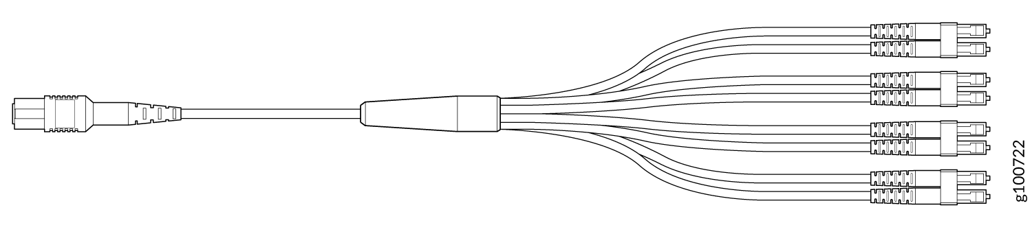
Table 4 describes the way the fibers are connected between the MPO and LC duplex connectors. The cable signals are the same as those described in Table 2.
|
MPO Connector Pin |
LC Duplex Connector Pin |
|---|---|
|
1 |
Tx on LC Duplex 1 |
|
2 |
Tx on LC Duplex 2 |
|
3 |
Tx on LC Duplex 3 |
|
4 |
Tx on LC Duplex 4 |
|
5 |
Unused |
|
6 |
Unused |
|
7 |
Unused |
|
8 |
Unused |
|
9 |
Rx on LC Duplex 4 |
|
10 |
Rx on LC Duplex 3 |
|
11 |
Rx on LC Duplex 2 |
|
12 |
Rx on LC Duplex 1 |
12-Ribbon Patch and Breakout Cables Available from Juniper Networks
Juniper Networks sells 12-ribbon patch and breakout cables with MPO connectors that meet the requirements described earlier. You are not required to purchase cables from Juniper Networks. Table 5 describes the available cables.
|
Cable Type |
Connector Type |
Fiber Type |
Cable Length |
Juniper Model Number |
|---|---|---|---|---|
|
12-ribbon patch |
Socket MPO/PC to socket MPO/PC, key up to key up |
MMF (OM3) |
1 m |
MTP12-FF-M1M |
|
3 m |
MTP12-FF-M3M |
|||
|
5 m |
MTP12-FF-M5M |
|||
|
10 m |
MTP12-FF-M10M |
|||
|
Socket MPO/APC to socket MPO/APC, key up to key up |
SMF |
1 m |
MTP12-FF-S1M |
|
|
3 m |
MTP12-FF-S3M |
|||
|
5 m |
MTP12-FF-S5M |
|||
|
10 m |
MTP12-FF-S10M |
|||
|
12-ribbon breakout |
Socket MPO/PC, key up, to four LC/UPC duplex |
MMF (OM3) |
1 m |
MTP-4LC-M1M |
|
3 m |
MTP-4LC-M3M |
|||
|
5 m |
MTP-4LC-M5M |
|||
|
10 m |
MTP-4LC-M10M |
|||
|
Socket MPO/APC, key up, to four LC/UPC duplex |
SMF |
1 m |
MTP-4LC-S1M |
|
|
3 m |
MTP-4LC-S3M |
|||
|
5 m |
MTP-4LC-S5M |
|||
|
10 m |
MTP-4LC-S10M |
24-Fiber MPO Connectors
You can use patch cables with 24-fiber MPO connectors to connect two supported transceivers of the same type—for example, 2x100GE-SR-to-2x100GE-SR.
Figure 2 shows the 24-fiber MPO optical lane assignments.
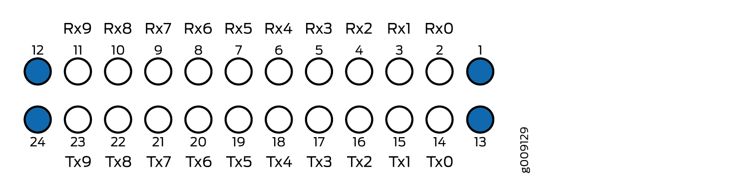
You must order cables with the correct polarity. Vendors refer to these crossover cables as key up to key up, latch up to latch up, Type B, or Method B. If you are using patch panels between two transceivers, ensure that the proper polarity is maintained through the cable plant.
16-Fiber MPO Connectors
You can use patch cables with 16-fiber MPO connectors to connect two supported transceivers of the same type. Figure 3 shows the optical plug and receptacle for one row MPO-16 connectors
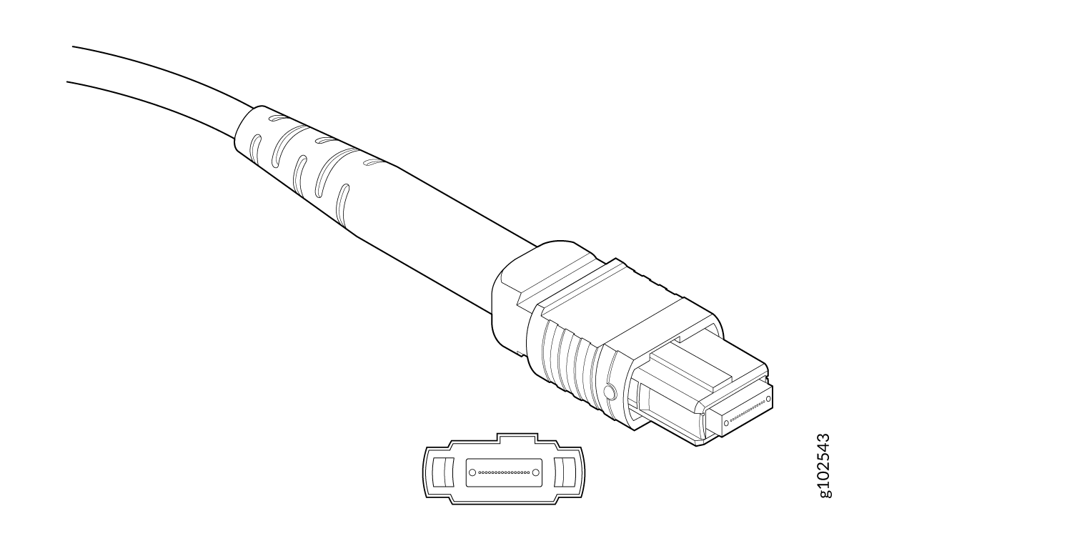
Table 6 lists the electrical signal to optical port mapping for QSFP-DD transceivers.
|
Electrical Data Input/Output |
MPO-12 (two row), MPO-16, or Dual MPO-12 |
MPO-12, MDC (BiDi) |
|---|---|---|
|
8 TX fibers and 8 RX fibers TX-n or RX-n where n is the optical port number as defined Figure 27. |
8 Tx (Rx) fibers TRn or RTn where n is the optical port number as defined Figure 27. |
|
|
Tx1 |
TX-1 |
TR1 |
|
Tx2 |
TX-2 |
RT1 |
|
Tx3 |
TX-3 |
TR2 |
|
Tx4 |
TX-4 |
RT2 |
|
Tx5 |
TX-5 |
TR3 |
|
Tx6 |
TX-6 |
RT3 |
|
Tx7 |
TX-7 |
TR4 |
|
Tx8 |
TX-8 |
RT4 |
|
Rx1 |
RX-1 |
RT1 |
|
Rx2 |
RX-2 |
TR1 |
|
Rx3 |
RX-3 |
RT2 |
|
Rx4 |
RX-4 |
TR2 |
|
Rx5 |
RX-5 |
RT3 |
|
Rx6 |
RX-6 |
TR3 |
|
Rx7 |
RX-7 |
RT4 |
|
Rx8 |
RX-8 |
TR4 |
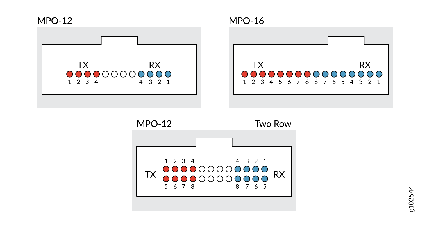
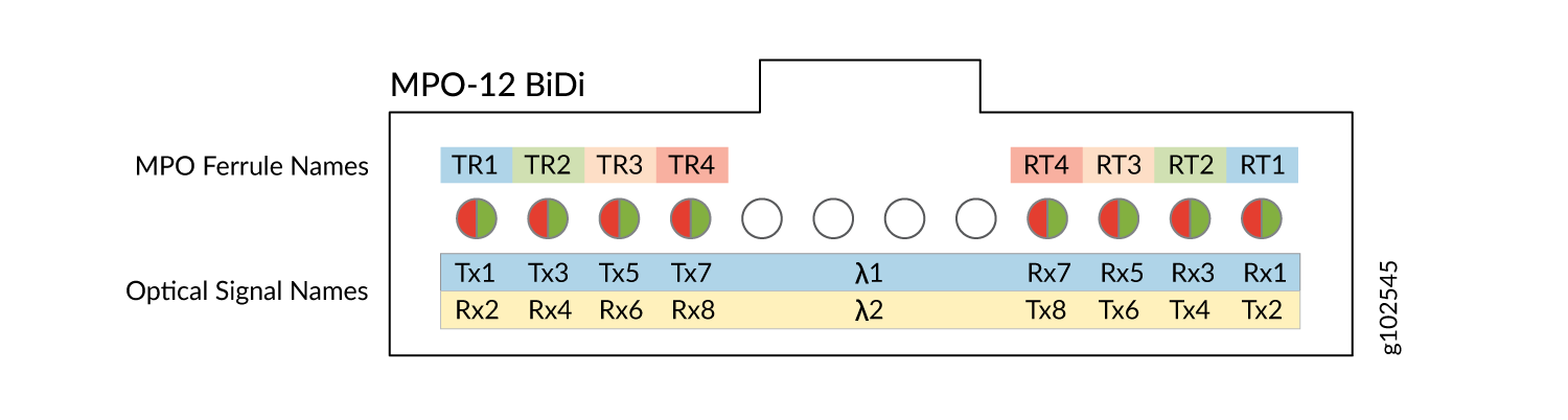
The MPO 12, 2 row optical MDI is used for breakout applications and is not intended for structured cabling applications.
CS Connector
You can use patch cables with CS connectors to connect two supported transceivers of the same type- for example, 2x100G-LR4 to 2x100G-LR4 or 2x100G-CWDM4 to 2x100G-CWDM4. CS connectors are compact connectors that are designed for next-generation QSFP-DD transceivers. The CS connector provides easy backward compatibility with QSFP28 and QSFP56 transceivers.
LC Duplex Connectors
You can use patch cables with LC duplex connectors to connect two supported transceivers of the same type—for example, 40GBASE-LR4-to-40GBASE-LR4 or 100GBASE-LR4-to 100GBASE-LR4. A patch cable is one fiber pair with two LC duplex connectors at opposite ends. LC duplex connectors are also used with 12-fiber ribbon breakout cables.
Figure 5 shows how to install an LC duplex connector in a transceiver.
Calculate Power Budget and Power Margin for Fiber-Optic Cables
Use the information in this topic and the specifications for your optical interface to calculate the power budget and power margin for fiber-optic cables.
You can use the Hardware Compatibility Tool to find information about the pluggable transceivers supported on your Juniper Networks device.
To calculate the power budget and power margin, perform the following tasks:
Calculate Power Budget for Fiber-Optic Cables
To ensure that fiber-optic connections have sufficient power for correct operation, you need to calculate the link's power budget (PB), which is the maximum amount of power it can transmit. When you calculate the power budget, you use a worst-case analysis to provide a margin of error, even though all the parts of an actual system do not operate at the worst-case levels. To calculate the worst-case estimate of PB, you assume minimum transmitter power (PT) and minimum receiver sensitivity (PR):
PB = PT – PR
The following hypothetical power budget equation uses values measured in decibels (dB) and decibels referred to one milliwatt (dBm):
PB = PT – PR
PB = –15 dBm – (–28 dBm)
PB = 13 dB
How to Calculate Power Margin for Fiber-Optic Cables
After calculating a link's PB, you can calculate the power margin (PM), which represents the amount of power available after subtracting attenuation or link loss (LL) from the PB. A worst-case estimate of PM assumes maximum LL:
PM = PB – LL
PM greater than zero indicates that the power budget is sufficient to operate the receiver.
Factors that can cause link loss include higher-order mode losses, modal and chromatic dispersion, connectors, splices, and fiber attenuation. Table 7 lists an estimated amount of loss for the factors used in the following sample calculations. For information about the actual amount of signal loss caused by equipment and other factors, refer to vendor documentation.
Link-Loss Factor |
Estimated Link-Loss Value |
|---|---|
Higher-order mode losses |
Single mode—None Multimode—0.5 dB |
Modal and chromatic dispersion |
Single mode—None Multimode—None, if product of bandwidth and distance is less than 500 MHz-km |
Faulty connector |
0.5 dB |
Splice |
0.5 dB |
Fiber attenuation |
Single mode—0.5 dB/km Multimode—1 dB/km |
The following sample calculation for a 2-km-long multimode link with a PB of 13 dB uses the estimated values from Table 7. This example calculates LL as the sum of fiber attenuation (2 km @ 1 dB/km, or 2 dB) and loss for five connectors (0.5 dB per connector, or 2.5 dB) and two splices (0.5 dB per splice, or 1 dB) as well as higher-order mode losses (0.5 dB). The PM is calculated as follows:
PM = PB – LL
PM = 13 dB – 2 km (1 dB/km) – 5 (0.5 dB) – 2 (0.5 dB) – 0.5 dB
PM = 13 dB – 2 dB – 2.5 dB – 1 dB – 0.5 dB
PM = 7 dB
The following sample calculation for an 8-km-long single-mode link with a PB of 13 dB uses the estimated values from Table 7. This example calculates LL as the sum of fiber attenuation (8 km @ 0.5 dB/km, or 4 dB) and loss for seven connectors (0.5 dB per connector, or 3.5 dB). The PM is calculated as follows:
PM = PB – LL
PM = 13 dB – 8 km (0.5 dB/km) – 7(0.5 dB)
PM = 13 dB – 4 dB – 3.5 dB
PM = 5.5 dB
In both the examples, the calculated PM is greater than zero, indicating that the link has sufficient power for transmission and does not exceed the maximum receiver input power.